3-Temperature-Model with Criticality#
Here, the NTM from the heat example is extended by a third subsystems for spins.
Reference
Khusyainov, D., Liefferink, R., et al., Time-resolved magnetic force microscopy of all-optical magnetization switching APL Mater. 14, 061109 (2026)
This leads to the following system of coupled differential equations:
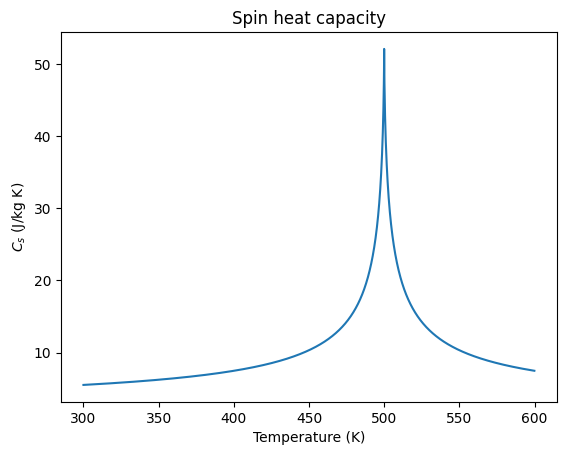
Moreover, to model critical behaviour of the spin heat capacity \(C_s(T)\) close to the Curie temperature \(T_C\), a phenomenological critical anomaly is of \(C_s(T)\) is introduced by:
The laser excitation is also modelled by \(i\) different laser pulse of variable delay, pulse width, and fluence.
Important
As in Khusyainov et al. the example is simplified by neglecting thermal diffusion and following an effective-medium approach for the metallic Co and Pt layers.
A full simulation including thermal conductivity is easily possible with the udkm1Dsim, but would require the careful determination of a large number of sub-system-dependent material parameters.
Setup#
Do all necessary imports and settings.
import udkm1Dsim as ud
u = ud.u  # import the pint unit registry from udkm1Dsim
import scipy.constants as constants
import numpy as np
import matplotlib.pyplot as plt
%matplotlib inline
u.setup_matplotlib()  # use matplotlib with pint units
Structure#
Refer to the structure example for more details.
Co = ud.Atom('Co')
Pt = ud.Atom('Pt')
Mg = ud.Atom('Mg')
O = ud.Atom('O')
Ta = ud.Atom('Ta')
Si = ud.Atom('Si')

SiO2 = ud.AtomMixed('SiO2')
SiO2.add_atom(Si, 0.33)
SiO2.add_atom(O, 0.67)

MgO = ud.AtomMixed('MgO')
MgO.add_atom(Mg, 0.5)
MgO.add_atom(O, 0.5)
Hint
Some parameters from Khusyaino, D., et al. are volume-specific while the udkm1Dsim toolbox requires mass-specific parameters.
density_effective = (8900*u.kg/u.m**3 + 10*21000*u.kg/u.m**3)/11

gamma = 2.6e2/density_effective.magnitude  # in J/kg/K²
C_s0 = 4e4/density_effective.magnitude  # in J/kg/K
zeta = 24.9
alpha = 0.7
T_c = 500
Delta = 5  # in K
G_el = 1.9e18  # in W/m³
G_es = 2.4e17  # in W/m³
G_sl = 3.0e15  # in W/m³

prop_Co = {}
prop_Co['heat_capacity'] = [f'{gamma:f}*T',
                            f'(2.98e6 + 1.5e3*(T-300))/{density_effective.magnitude:f}',
                            f'{C_s0:f}*(1+{zeta:f}/(1+abs((T-{T_c:f})/{Delta:f})**{alpha:f}))'
                           ]

# only allow for electronic conduction to equilibrate Co and Pt
prop_Co['therm_cond'] = [1000, 0, 0]

prop_Co['sub_system_coupling'] = \
    [f'-{G_el:f}*(T_0-T_1)-{G_es:f}*(T_0-T_2)',
     f'-{G_el:f}*(T_1-T_0)-{G_sl:f}*(T_1-T_2)',
     f'-{G_es:f}*(T_2-T_0)-{G_sl:f}*(T_2-T_1)',
    ]
prop_Co['lin_therm_exp'] = [0, 0, 0]
prop_Co['opt_ref_index'] = 2.5+4.8j

layer_Co = ud.AmorphousLayer('Co', 'Co layer', thickness=0.1*u.nm,
                             density=density_effective, atom=Co, **prop_Co)
Number of subsystems changed from 1 to 3.
/home/schick/Programming/git/udkm1Dsim/udkm1Dsim/structures/layers.py:499: UserWarning:
The sympy integration of the heat capacity did not work. It is only required for

    Heat.get_temperature_after_delta_excitation()

You can set its analytical anti-derivative manually as a str representing the correct function of temperature T by typing

    layer.int_heat_capacity = 'c(T)'

where layer is the name of the layer object.

  warnings.warn('\nThe sympy integration of the heat capacity did not work. '
Important
The UserWarning above is not relevant for this example when calculating heat diffusion with a finite pulse duration.
prop_Pt = {}
prop_Pt['heat_capacity'] = prop_Co['heat_capacity']
prop_Pt['therm_cond'] = prop_Co['therm_cond']
prop_Pt['sub_system_coupling'] = prop_Co['sub_system_coupling']
prop_Pt['lin_therm_exp'] = [0, 0, 0]
prop_Pt['opt_ref_index'] = 2.7254+6.1280j  # A. Tselin, et al., Phys. Rev. B 110, 195130 (2024)

layer_Pt = ud.AmorphousLayer('Pt', 'Pt layer', 0.1*u.nm, density_effective, atom=Pt, **prop_Pt)
Number of subsystems changed from 1 to 3.
prop_Ta = {}
prop_Ta['heat_capacity'] = [40*u.J/u.kg/u.K, 100*u.J/u.kg/u.K, 1e-6]
prop_Ta['therm_cond'] = [0, 0, 0]
prop_Ta['sub_system_coupling'] = ['5e17*(T_1-T_0)',
                                  '5e17*(T_0-T_1)',
                                  0]
prop_Ta['lin_therm_exp'] = [0, 0, 0]
prop_Ta['opt_ref_index'] = 1.111+3.4796j

layer_Ta = ud.AmorphousLayer('Ta', 'Ta layer', thickness=0.1*u.nm, density=16650*u.kg/u.m**3,
                              atom=Ta, **prop_Ta)
Number of subsystems changed from 1 to 3.
prop_Al = {}
prop_Al['heat_capacity'] = [200*u.J/u.kg/u.K, 700*u.J/u.kg/u.K, 1e-6]
prop_Al['therm_cond'] = [0, 0, 0]
prop_Al['sub_system_coupling'] = ['5e17*(T_1-T_0)',
                                  '5e17*(T_0-T_1)',
                                  0]
prop_Al['lin_therm_exp'] = [0, 0, 0]
prop_Al['opt_ref_index'] = 2.767+8.354j

layer_Al = ud.AmorphousLayer('Al', 'Al layer', thickness=0.1*u.nm, density=2700*u.kg/u.m**3,
                                atom=SiO2, **prop_Al)
Number of subsystems changed from 1 to 3.
prop_MgO = {}
prop_MgO['heat_capacity'] = [1e-6, 923*u.J/u.kg/u.K, 1e-6]
prop_MgO['therm_cond'] = [0, 0, 0]
prop_MgO['sub_system_coupling'] = [0, 0, 0]
prop_MgO['lin_therm_exp'] = [0, 0, 0]
prop_MgO['opt_ref_index'] = 1.72+0.0j

layer_MgO = ud.AmorphousLayer('MgO', 'MgO laser', thickness=0.1*u.nm, density=3580*u.kg/u.m**3,
                                atom=SiO2, **prop_MgO)
Number of subsystems changed from 1 to 3.
prop_glass = {}
prop_glass['heat_capacity'] = [1e-6, 700*u.J/u.kg/u.K, 1e-6]
prop_glass['therm_cond'] = [0, 0, 0]
prop_glass['sub_system_coupling'] = [0, 0, 0]
prop_glass['lin_therm_exp'] = [0, 0, 0]
prop_glass['opt_ref_index'] = 3.6941+0.0

layer_glass = ud.AmorphousLayer('glass', 'glass laser', thickness=1*u.nm, density=2650*u.kg/u.m**3,
                                atom=SiO2, **prop_glass)
Number of subsystems changed from 1 to 3.
S = ud.Structure('Sample')

S.add_sub_structure(layer_Ta, 10)
S.add_sub_structure(layer_MgO, 20)
S.add_sub_structure(layer_Pt, 30)
S.add_sub_structure(layer_Co, 6)
S.add_sub_structure(layer_Pt, 30)
S.add_sub_structure(layer_Ta, 40)
S.add_sub_structure(layer_glass, 10)
S.visualize()

Initialize Heat and the Excitation#
h = ud.Heat(S, True)

h.save_data = False
h.disp_messages = True

# enable heat diffusion
h.heat_diffusion = True
# set the boundary conditions
h.boundary_conditions = {'top_type': 'isolator', 'bottom_type': 'isolator'}
# spatial grid
_, _, distances = S.get_distances_of_layers()
# select only Co and Pt layers for plotting
select = np.concat((S.get_all_positions_per_unique_layer()['Co'], S.get_all_positions_per_unique_layer()['Pt']))
delays = np.r_[-2.5:10:0.01]*u.ps

fluence = 3.5  # in mJ/cm²
Criticallity of Spin Heat Capacity#
temps = np.r_[300:600:0.1]

plt.figure()
plt.plot(temps, layer_Co.heat_capacity[2](temps))
plt.xlabel('Temperature (K)')
plt.ylabel('$C_s$ (J/kg K)')
plt.title('Spin heat capacity')
plt.show()
Absorption profile#
plt.figure()
dAdz, _, _, _ = h.get_multilayers_absorption_profile()
plt.stairs(dAdz[:-1], distances.to('nm'))
plt.xlabel('Distance (nm)')
plt.ylabel('Differnetial Absorption')
plt.title('Laser Absorption Profile')
plt.show()
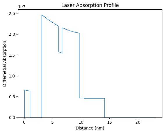
Absorption profile is calculated by multilayer formalism with p-polarization.
Total reflectivity of 55.5 % and transmission of 27.9 %.
Single-Pulse Excitation#
100-fs-Pulse#
h.excitation = {'fluence': [fluence]*u.mJ/u.cm**2,
                'delay_pump':  [0]*u.ps,
                'pulse_width':  [0.1/2.355]*u.ps,  # from FWHM to sigma
                'multilayer_absorption': True,
                'wavelength': 800*u.nm,
                'theta': 90*u.deg}

temp_map_100fs, delta_temp_100fs = h.get_temp_map(delays, 300)
Surface incidence fluence scaled by factor 1.0000 due to incidence angle theta=90.00 deg
Calculating _heat_diffusion_ for excitation 1:1 ...
Absorption profile is calculated by multilayer formalism with p-polarization.
Total reflectivity of 55.5 % and transmission of 27.9 %.
Elapsed time for _heat_diffusion_ with 1 excitation(s): 29.174119 s
Calculating _heat_diffusion_ without excitation...
Elapsed time for _heat_diffusion_: 32.456030 s
Elapsed time for _temp_map_: 61.733104 s
3-ps-Pulse#
h.excitation = {'fluence': [fluence]*u.mJ/u.cm**2,
                'delay_pump':  [0]*u.ps,
                'pulse_width':  [3.0/2.355]*u.ps,  # from FWHM to sigma
                'multilayer_absorption': True,
                'wavelength': 800*u.nm,
                'theta': 90*u.deg}

temp_map_3ps, delta_temp_3ps = h.get_temp_map(delays, 300)
Surface incidence fluence scaled by factor 1.0000 due to incidence angle theta=90.00 deg
Calculating _heat_diffusion_ for excitation 1:1 ...
Absorption profile is calculated by multilayer formalism with p-polarization.
Total reflectivity of 55.5 % and transmission of 27.9 %.
Elapsed time for _heat_diffusion_ with 1 excitation(s): 25.596356 s
Calculating _heat_diffusion_ without excitation...
Elapsed time for _heat_diffusion_: 8.841166 s
Elapsed time for _temp_map_: 34.568653 s
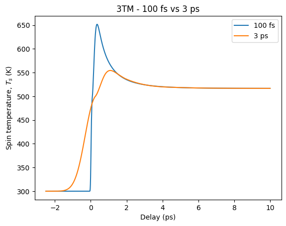
Comparison of Spin temperatures#
plt.figure()
plt.plot(delays.to('ps'), np.mean(temp_map_100fs[:, select, 2], 1), label='100 fs')
plt.plot(delays.to('ps'), np.mean(temp_map_3ps[:, select, 2], 1), label='3 ps')
plt.ylabel('Spin temperature, $T_s$ (K)')
plt.xlabel('Delay (ps)')
plt.legend()
plt.title('3TM - 100 fs vs 3 ps')
plt.show()
Double Pulse Excitation#
Hint
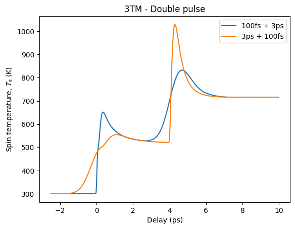
Multipluse excitation is readily available by the providing lists of fluence, delay_pump, and pulse_width of the excitation dictionary.
100 fs + 3 ps#
h.excitation = {'fluence': [fluence, fluence]*u.mJ/u.cm**2,
                'delay_pump':  [0, 4]*u.ps,
                'pulse_width':  [0.1, 3]*u.ps/2.355,
                'multilayer_absorption': True,
                'wavelength': 800*u.nm,
                'theta': 90*u.deg}

temp_map_100fs_3ps, delta_temp_100fs_3ps = h.get_temp_map(delays, 300)
Surface incidence fluence scaled by factor 1.0000 due to incidence angle theta=90.00 deg
Calculating _heat_diffusion_ for excitation 1:2 ...
Absorption profile is calculated by multilayer formalism with p-polarization.
Total reflectivity of 55.5 % and transmission of 27.9 %.
Elapsed time for _heat_diffusion_ with 1 excitation(s): 14.132894 s
Calculating _heat_diffusion_ without excitation...
Elapsed time for _heat_diffusion_: 26.430818 s
Calculating _heat_diffusion_ for excitation 2:2 ...
Absorption profile is calculated by multilayer formalism with p-polarization.
Total reflectivity of 55.5 % and transmission of 27.9 %.
Elapsed time for _heat_diffusion_ with 1 excitation(s): 20.259503 s
Calculating _heat_diffusion_ without excitation...
Elapsed time for _heat_diffusion_: 8.812536 s
Elapsed time for _temp_map_: 69.786765 s
3 ps + 100 fs#
h.excitation = {'fluence': [fluence, fluence]*u.mJ/u.cm**2,
                'delay_pump':  [0, 4]*u.ps,
                'pulse_width':  [3, 0.1]*u.ps/2.355,
                'multilayer_absorption': True,
                'wavelength': 800*u.nm,
                'theta': 90*u.deg}

temp_map_3ps_100fs, delta_temp_3ps_100fs = h.get_temp_map(delays, 300)
Surface incidence fluence scaled by factor 1.0000 due to incidence angle theta=90.00 deg
Calculating _heat_diffusion_ for excitation 1:2 ...
Absorption profile is calculated by multilayer formalism with p-polarization.
Total reflectivity of 55.5 % and transmission of 27.9 %.
Elapsed time for _heat_diffusion_ with 1 excitation(s): 32.957248 s
Calculating _heat_diffusion_ without excitation...
Elapsed time for _heat_diffusion_: 1.723398 s
Calculating _heat_diffusion_ for excitation 2:2 ...
Absorption profile is calculated by multilayer formalism with p-polarization.
Total reflectivity of 55.5 % and transmission of 27.9 %.
Elapsed time for _heat_diffusion_ with 1 excitation(s): 21.719136 s
Calculating _heat_diffusion_ without excitation...
Elapsed time for _heat_diffusion_: 26.382524 s
Elapsed time for _temp_map_: 82.972926 s
Comparison#
plt.figure()
plt.plot(delays.to('ps'), np.mean(temp_map_100fs_3ps[:, select, 2], 1), label='100fs + 3ps')
plt.plot(delays.to('ps'), np.mean(temp_map_3ps_100fs[:, select, 2], 1), label='3ps + 100fs')
plt.ylabel('Spin temperature, $T_s$ (K)')
plt.xlabel('Delay (ps)')
plt.legend()
plt.title('3TM - Double pulse')
plt.show()
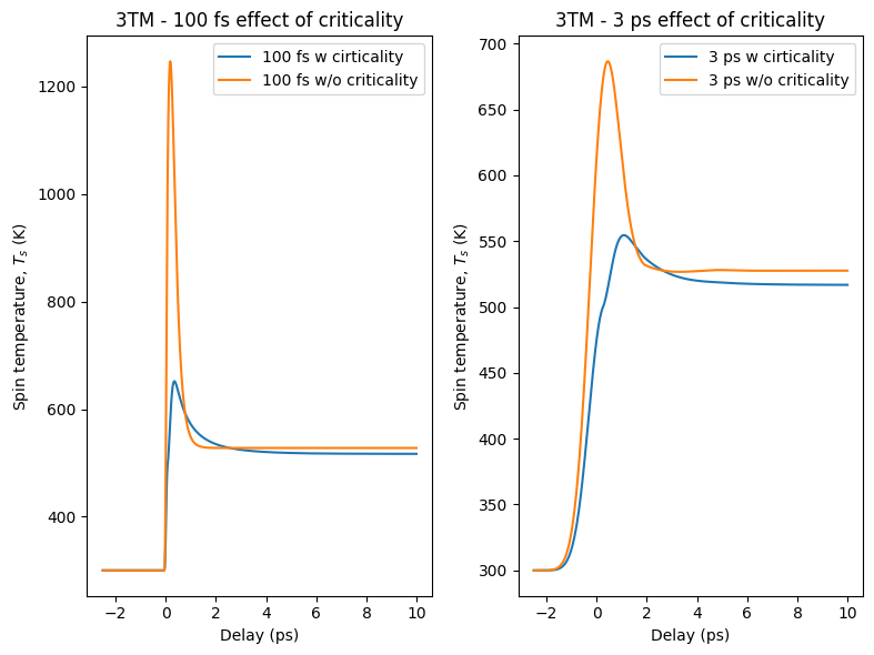
Effect of Criticality#
layer_Co.heat_capacity = [f'{gamma:f}*T',
                          f'(2.98e6 + 1.5e3*(T-300))/{density_effective.magnitude:f}',
                          f'{C_s0:f}'
                          ]

layer_Pt.heat_capacity = [f'{gamma:f}*T',
                          f'(2.98e6 + 1.5e3*(T-300))/{density_effective.magnitude:f}',
                          f'{C_s0:f}'
                          ]
h.excitation = {'fluence': [fluence]*u.mJ/u.cm**2,
                'delay_pump':  [0]*u.ps,
                'pulse_width':  [0.1/2.355]*u.ps,  # from FWHM to sigma
                'multilayer_absorption': True,
                'wavelength': 800*u.nm,
                'theta': 90*u.deg}

temp_map_100fs_wo_crit, delta_temp_100fs_wo_crit = h.get_temp_map(delays, 300)
Surface incidence fluence scaled by factor 1.0000 due to incidence angle theta=90.00 deg
Calculating _heat_diffusion_ for excitation 1:1 ...
Absorption profile is calculated by multilayer formalism with p-polarization.
Total reflectivity of 55.5 % and transmission of 27.9 %.
Elapsed time for _heat_diffusion_ with 1 excitation(s): 13.192575 s
Calculating _heat_diffusion_ without excitation...
Elapsed time for _heat_diffusion_: 28.466990 s
Elapsed time for _temp_map_: 41.793093 s
h.excitation = {'fluence': [fluence]*u.mJ/u.cm**2,
                'delay_pump':  [0]*u.ps,
                'pulse_width':  [3.0/2.355]*u.ps,  # from FWHM to sigma
                'multilayer_absorption': True,
                'wavelength': 800*u.nm,
                'theta': 90*u.deg}

temp_map_3ps_wo_crit, delta_temp_3ps_wo_crit = h.get_temp_map(delays, 300)
Surface incidence fluence scaled by factor 1.0000 due to incidence angle theta=90.00 deg
Calculating _heat_diffusion_ for excitation 1:1 ...
Absorption profile is calculated by multilayer formalism with p-polarization.
Total reflectivity of 55.5 % and transmission of 27.9 %.
Elapsed time for _heat_diffusion_ with 1 excitation(s): 14.999972 s
Calculating _heat_diffusion_ without excitation...
Elapsed time for _heat_diffusion_: 3.662041 s
Elapsed time for _temp_map_: 18.780535 s
Comparison#
plt.figure(figsize=[8, 6])
plt.subplot(1, 2, 1)
plt.plot(delays.to('ps'), np.mean(temp_map_100fs[:, select, 2], 1), label='100 fs w cirticality')
plt.plot(delays.to('ps'), np.mean(temp_map_100fs_wo_crit[:, select, 2], 1), label='100 fs w/o criticality')
plt.ylabel('Spin temperature, $T_s$ (K)')
plt.xlabel('Delay (ps)')
plt.legend()
plt.title('3TM - 100 fs effect of criticality')

plt.subplot(1, 2, 2)
plt.plot(delays.to('ps'), np.mean(temp_map_3ps[:, select, 2], 1), label='3 ps w cirticality')
plt.plot(delays.to('ps'), np.mean(temp_map_3ps_wo_crit[:, select, 2], 1), label='3 ps w/o criticality')
plt.ylabel('Spin temperature, $T_s$ (K)')
plt.xlabel('Delay (ps)')
plt.legend()
plt.title('3TM - 3 ps effect of criticality')

plt.tight_layout()
plt.show()