Dynamical Magnetic X-ray Scattering

In this example static and transient magnetic X-ray simulations are carried out employing a dynamical magnetic X-ray scattering formalism which was adapted from Project Dyna.

Setup

Do all necessary imports and settings.

import udkm1Dsim as ud
u = ud.u  # import the pint unit registry from udkm1Dsim
import numpy as np
import matplotlib.pyplot as plt
%matplotlib inline
u.setup_matplotlib()  # use matplotlib with pint units

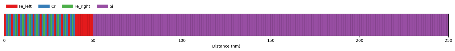
Structure

Refer to the structure-example for more details.

In this example the sample Structure consists of AmorphousLayers.

In order to build an antiferromagnetic sample two different types of Fe Atoms and AmorphousLayers are created with opposite in-plane magnetization.

Here a local file for the atomic scattering factor is read only for Fe atoms.

Fe_right = ud.Atom('Fe', mag_amplitude=1, mag_phi=90*u.deg, mag_gamma=90*u.deg,
                   atomic_form_factor_path='./Fe.cf')
Fe_left = ud.Atom('Fe', mag_amplitude=1, mag_phi=90*u.deg, mag_gamma=270*u.deg,
                  atomic_form_factor_path='./Fe.cf')
Cr = ud.Atom('Cr')
Si = ud.Atom('Si')

density_Fe = 7874*u.kg/u.m**3

prop_Fe = {}
prop_Fe['heat_capacity'] = 449*u.J/u.kg/u.K
prop_Fe['therm_cond'] = 80*u.W/(u.m *u.K)
prop_Fe['lin_therm_exp'] = 11.8e-6
prop_Fe['sound_vel'] = 4.910*u.nm/u.ps
prop_Fe['opt_ref_index'] = 2.9174+3.3545j

layer_Fe_left = ud.AmorphousLayer('Fe_left', 'Fe left amorphous', 1*u.nm,
                                  density_Fe, atom=Fe_left, **prop_Fe)
layer_Fe_right = ud.AmorphousLayer('Fe_right', 'Fe right amorphous', 1*u.nm,
                                   density_Fe, atom=Fe_right, **prop_Fe)

density_Cr = 7140*u.kg/u.m**3

prop_Cr = {}
prop_Cr['heat_capacity'] = 449*u.J/u.kg/u.K
prop_Cr['therm_cond'] = 94*u.W/(u.m*u.K)
prop_Cr['lin_therm_exp'] = 6.2e-6
prop_Cr['sound_vel'] = 5.940*u.nm/u.ps
prop_Cr['opt_ref_index'] = 3.1612+3.4606j

layer_Cr = ud.AmorphousLayer('Cr', "Cr amorphous", 1*u.nm, density_Cr, atom=Cr, **prop_Cr)

density_Si = 2336*u.kg/u.m**3

prop_Si = {}
prop_Si['heat_capacity'] = 703*u.J/u.kg/u.K
prop_Si['therm_cond'] = 150*u.W/(u.m*u.K)
prop_Si['lin_therm_exp'] = 2.6e-6
prop_Si['sound_vel'] = 8.433*u.nm/u.ps
prop_Si['opt_ref_index'] = 3.6941+0.0065435j

layer_Si = ud.AmorphousLayer('Si', "Si amorphous", 1*u.nm, density_Si, atom=Si, **prop_Si)

S = ud.Structure('Fe/Cr AFM Super Lattice')

# create a sub-structure
DL = ud.Structure('Two Fe/Cr Double Layers')
DL.add_sub_structure(layer_Fe_left, 1)
DL.add_sub_structure(layer_Cr, 1)
DL.add_sub_structure(layer_Fe_right, 1)
DL.add_sub_structure(layer_Cr, 1)

S.add_sub_structure(DL, 10)
S.add_sub_structure(layer_Fe_left, 10)
S.add_sub_structure(layer_Si, 200)

S.visualize()

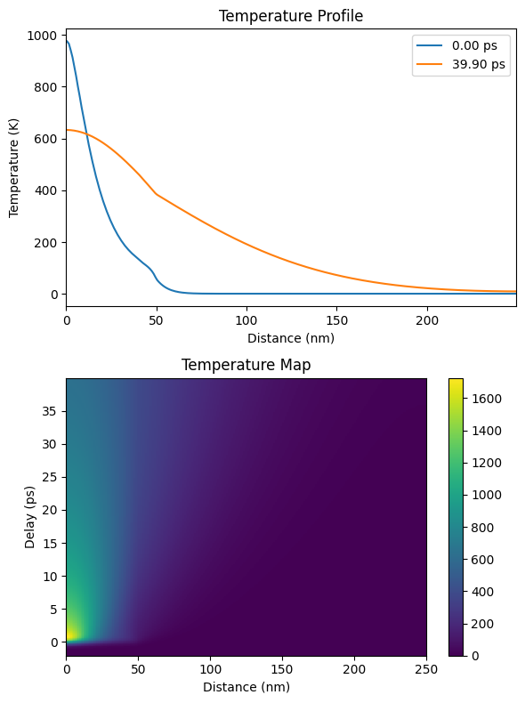
Heat

Refer to the heat-example for more details.

h = ud.Heat(S, True)

h.save_data = False
h.disp_messages = True

h.excitation = {'fluence': [40]*u.mJ/u.cm**2,
                'delay_pump':  [0]*u.ps,
                'pulse_width':  [1]*u.ps,
                'multilayer_absorption': True,
                'wavelength': 800*u.nm,
                'theta': 45*u.deg}

# enable heat diffusion
h.heat_diffusion = True

# temporal and spatial grid
delays = np.r_[-2:40:0.1]*u.ps
_, _, distances = S.get_distances_of_layers()

temp_map, delta_temp_map = h.get_temp_map(delays, 0*u.K)

Surface incidence fluence scaled by factor 0.7071 due to incidence angle theta=45.00 deg
Calculating _heat_diffusion_ for excitation 1:1 ...
Absorption profile is calculated by multilayer formalism.
Total reflectivity of 47.7 % and transmission of 6.4 %.

Elapsed time for _heat_diffusion_ with 1 excitation(s): 21.034174 s
Calculating _heat_diffusion_ without excitation...

Elapsed time for _heat_diffusion_: 11.240211 s
Elapsed time for _temp_map_: 32.503744 s

plt.figure(figsize=[6, 8])
plt.subplot(2, 1, 1)
plt.plot(distances.to('nm').magnitude, temp_map[20, :],
         label='{:0.2f} ps'.format(delays[20].to('ps').magnitude))
plt.plot(distances.to('nm').magnitude, temp_map[-1, :],
         label='{:0.2f} ps'.format(delays[-1].to('ps').magnitude))
plt.xlim([0, distances.to('nm').magnitude[-1]])
plt.xlabel('Distance [nm]')
plt.ylabel('Temperature [K]')
plt.legend()
plt.title('Temperature Profile')

plt.subplot(2, 1, 2)
plt.pcolormesh(distances.to('nm').magnitude, delays.to('ps').magnitude, temp_map, shading='auto')
plt.colorbar()
plt.xlabel('Distance [nm]')
plt.ylabel('Delay [ps]')
plt.title('Temperature Map')

plt.tight_layout()
plt.show()

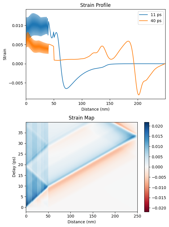
Numerical Phonons

Refer to the phonons-example for more details.

p = ud.PhononNum(S, True)
p.save_data = False
p.disp_messages = True

strain_map = p.get_strain_map(delays, temp_map, delta_temp_map)

Calculating linear thermal expansion ...
Calculating coherent dynamics with ODE solver ...

Elapsed time for _strain_map_: 0.717197 s

plt.figure(figsize=[6, 8])
plt.subplot(2, 1, 1)
plt.plot(distances.to('nm').magnitude, strain_map[130, :], label=np.round(delays[130]))
plt.plot(distances.to('nm').magnitude, strain_map[-1, :], label=np.round(delays[-1]))
plt.xlim([0, distances.to('nm').magnitude[-1]])
plt.xlabel('Distance [nm]')
plt.ylabel('Strain')
plt.legend()
plt.title('Strain Profile')

plt.subplot(2, 1, 2)
plt.pcolormesh(distances.to('nm').magnitude, delays.to('ps').magnitude,
               strain_map, cmap='RdBu', vmin=-np.max(strain_map),
               vmax=np.max(strain_map), shading='auto')
plt.colorbar()
plt.xlabel('Distance [nm]')
plt.ylabel('Delay [ps]')
plt.title('Strain Map')

plt.tight_layout()
plt.show()

Magnetization

The Magnetization class is currently only an interface to allow the user for defining specific magnetization dynamics depending on the strain_map and temp_map.

Here the magnetization as function of temperature is used as a simplified model to alter the transient magnetization amplitude.

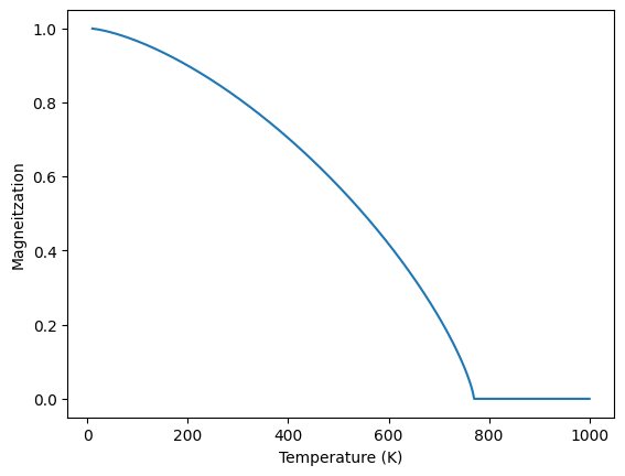
def magnetization_bloch(x, Tc, M0, beta):
    m = M0*((1-(x/Tc)**(3/2))*np.heaviside(Tc-x, 0.5))**beta
    return m


plt.figure()
temperatures = np.r_[10:1000:0.1]
plt.plot(temperatures, magnetization_bloch(temperatures, 770, 1, 0.75))
plt.xlabel('Temperature [K]')
plt.ylabel('Magneitzation')
plt.show()

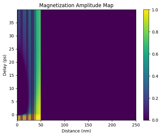
The calc_magnetization_map method must be overwritten to allow for calculating magnetization dynamics.

class SimpleMagnetization(ud.Magnetization):

    def calc_magnetization_map(self, delays, **kwargs):
        temp_map = kwargs['temp_map']
        T_c = kwargs['T_c']
        magnetization_map = np.zeros([len(delays),
                                      self.S.get_number_of_layers(), 3])
        handles = self.S.get_layer_vectors()[2]

        for i, handle in enumerate(handles):
            if handle.id in ['Fe_left', 'Fe_right']:
                magnetization_map[:, i, 0] = magnetization_bloch(temp_map[:, i], T_c, 1, .75)
            handle.magnetization['phi']
            magnetization_map[:, i, 1] = handle.magnetization['phi'].to_base_units().magnitude
            magnetization_map[:, i, 2] = handle.magnetization['gamma'].to_base_units().magnitude

        return magnetization_map

mag = SimpleMagnetization(S, True)
mag.save_data = False

magnetization_map = mag.get_magnetization_map(delays,
                                              strain_map=strain_map,
                                              temp_map=temp_map,
                                              T_c=770)

Calculating _magnetization_map_ ...
Elapsed time for _magnetization_map_: 0.021199 s

plt.figure()
plt.pcolormesh(distances.to('nm').magnitude, delays.to('ps').magnitude,
               magnetization_map[:, :, 0], shading='auto')
plt.title('Magnetization Amplitude Map')
plt.ylabel('Delay [ps]')
plt.xlabel('Distance [nm]')
plt.colorbar()
plt.show()

Initialize dynamical magnetic X-ray simulations

The XrayDynMag class requires a Structure object and a boolean force_recalc in order overwrite previous simulation results.

These results are saved in the cache_dir when save_data is enabled. Printing simulation messages can be en-/disabled using disp_messages and progress bars can using the boolean switch progress_bar.

dyn_mag = ud.XrayDynMag(S, True)
dyn_mag.disp_messages = True
dyn_mag.save_data = False

incoming polarizations set to: sigma
analyzer polarizations set to: unpolarized

Homogeneous magnetic X-ray scattering

For the case of homogeneously strained/magnetized samples, the dynamical magnetic X-ray scattering simulations can be greatly simplified, which saves a lot of computational time.

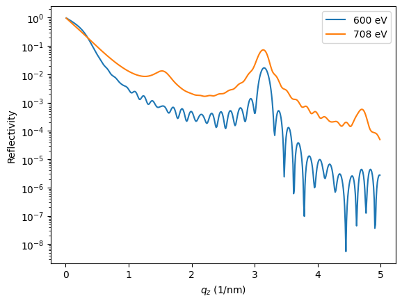
\(q_z\)-scan

The XrayDynMag object requires an energy and scattering vector qz to run the simulations.
Both parameters can be arrays and the resulting reflectivity has a first dimension for the photon energy and the a second for the scattering vector.

The resulting reflectivity is always calculated for the actual magnetization (R_hom) of the sample, as well as for opposite magnetization (R_hom_phi).

dyn_mag.energy = np.r_[600, 708]*u.eV  # set two photon energies
dyn_mag.qz = np.r_[0.01:5:0.01]/u.nm  # qz range
# this is the actual calculation
R_hom, R_hom_phi, _, _ = dyn_mag.homogeneous_reflectivity()

Calculating _homogeneous_reflectivity_ ...
Elapsed time for _homogeneous_reflectivity_: 0.715025 s

In this example half-order antiferromagnetic Bragg peaks appear only at the resonance.

plt.figure()
plt.semilogy(dyn_mag.qz[0, :], R_hom[0, :], label='{}'.format(dyn_mag.energy[0]))
plt.semilogy(dyn_mag.qz[1, :], R_hom[1, :], label='{}'.format(dyn_mag.energy[1]))
plt.ylabel('Reflectivity')
plt.xlabel(r'$q_z$ [1/nm]')
plt.legend()
plt.show()

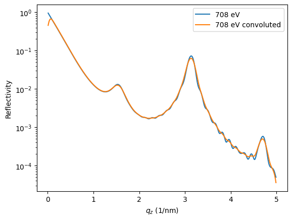
Post-Processing

Simple convolution of the results with an arbitrary function handle.

FWHM = 0.01/1e-10  # Angstrom
sigma = FWHM/2.3548

handle = lambda x: np.exp(-((x)/sigma)**2/2)
y_conv = dyn_mag.conv_with_function(R_hom[1, :], dyn_mag._qz[1, :], handle)

plt.figure()
plt.semilogy(dyn_mag.qz[0, :], R_hom[1, :], label='{}'.format(dyn_mag.energy[1]))
plt.semilogy(dyn_mag.qz[0, :], y_conv, label='{} convoluted'.format(dyn_mag.energy[1]))
plt.ylabel('Reflectivity')
plt.legend()
plt.show()

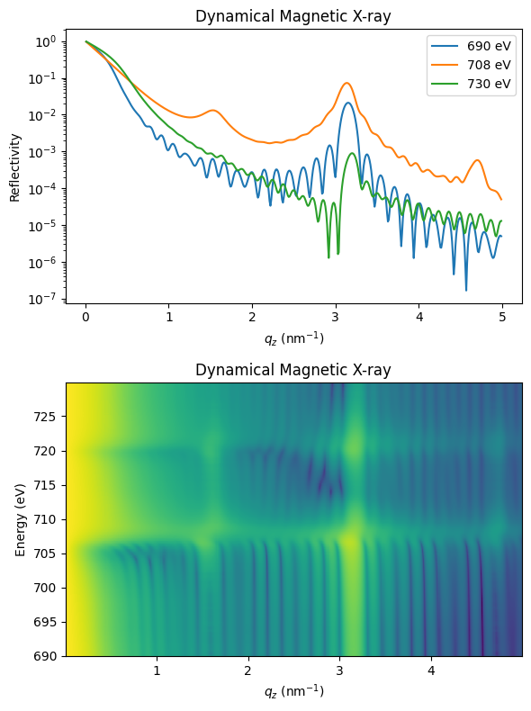
Energy- and \(q_z\)-scan

dyn_mag.energy = np.r_[690:730:0.1]*u.eV  # set the energy range
dyn_mag.qz = np.r_[0.01:5:0.01]/u.nm  # qz range
# this is the actual calculation
R_hom, R_hom_phi, _, _ = dyn_mag.homogeneous_reflectivity()

Calculating _homogeneous_reflectivity_ ...
Elapsed time for _homogeneous_reflectivity_: 141.994139 s

plt.figure(figsize=[6, 8])
plt.subplot(2, 1, 1)
plt.semilogy(dyn_mag.qz[0, :].to('1/nm'), R_hom[0, :],
             label=np.round(dyn_mag.energy[0]))
plt.semilogy(dyn_mag.qz[0, :].to('1/nm'), R_hom[180, :],
             label=np.round(dyn_mag.energy[180]))
plt.semilogy(dyn_mag.qz[0, :].to('1/nm'), R_hom[-1, :],
             label=np.round(dyn_mag.energy[-1]))

plt.xlabel('$q_z$ [nm$^{-1}$]')
plt.ylabel('Reflectivity')
plt.legend()
plt.title('Dynamical Magnetic X-ray')

plt.subplot(2, 1, 2)
plt.pcolormesh(dyn_mag.qz[0, :].to('1/nm').magnitude, dyn_mag.energy.magnitude,
               np.log10(R_hom[:, :]), shading='auto')
plt.title('Dynamical Magnetic X-ray')
plt.ylabel('Energy [eV]')
plt.xlabel('$q_z$ [nm$^{-1}$]')

plt.tight_layout()
plt.show()

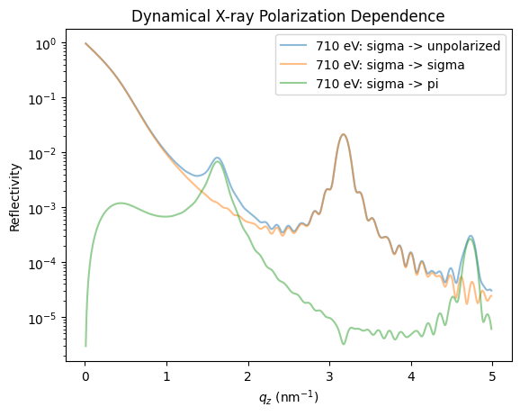
Polarization dependence

The XrayDynMag allows to set the incoming and outgoing polarization of the X-rays.

dyn_mag.energy = np.r_[710]*u.eV  # set two photon energies
dyn_mag.qz = np.r_[0.01:5:0.01]/u.nm  # qz range

plt.figure()
dyn_mag.set_polarization(3, 0)
R_hom, R_hom_phi, _, _ = dyn_mag.homogeneous_reflectivity()
plt.semilogy(dyn_mag.qz[0, :], R_hom[0, :],
             label='{}: sigma -> unpolarized'.format(dyn_mag.energy[0]),
             alpha=0.5)

dyn_mag.set_polarization(3, 3)
R_hom, R_hom_phi, _, _ = dyn_mag.homogeneous_reflectivity()
plt.semilogy(dyn_mag.qz[0, :], R_hom[0, :],
             label='{}: sigma -> sigma'.format(dyn_mag.energy[0]), alpha=0.5)

dyn_mag.set_polarization(3, 4)
R_hom, R_hom_phi, _, _ = dyn_mag.homogeneous_reflectivity()
plt.semilogy(dyn_mag.qz[0, :], R_hom[0, :],
             label='{}: sigma -> pi'.format(dyn_mag.energy[0]), alpha=0.5)

plt.xlabel('$q_z$ [nm$^{-1}$]')
plt.ylabel('Reflectivity')
plt.title('Dynamical X-ray Polarization Dependence')
plt.legend()
plt.show()

incoming polarizations set to: sigma
analyzer polarizations set to: unpolarized
Calculating _homogeneous_reflectivity_ ...
Elapsed time for _homogeneous_reflectivity_: 0.480793 s
incoming polarizations set to: sigma
analyzer polarizations set to: sigma
Calculating _homogeneous_reflectivity_ ...
Elapsed time for _homogeneous_reflectivity_: 0.379073 s
incoming polarizations set to: sigma
analyzer polarizations set to: pi
Calculating _homogeneous_reflectivity_ ...
Elapsed time for _homogeneous_reflectivity_: 0.361267 s

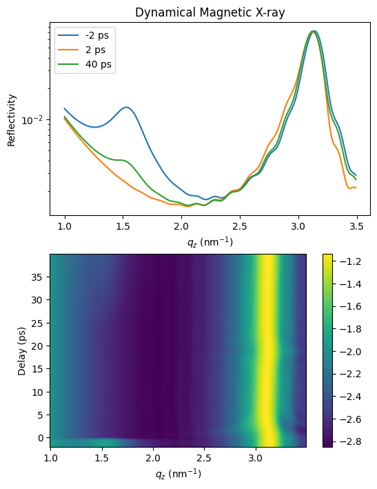
Inhomogeneous dynamical magnetic X-ray scattering

The inhomogeneous_reflectivity() method allows to calculate the transient magnetic X-ray reflectivity according to a strain_map and/or magnetization_map.

dyn_mag.energy = np.r_[708]*u.eV  # set the energy range
dyn_mag.qz = np.r_[1:3.5:0.01]/u.nm  # qz range
dyn_mag.set_polarization(3, 0)

incoming polarizations set to: sigma
analyzer polarizations set to: unpolarized

R_seq, R_seq_phi, _, _ = dyn_mag.inhomogeneous_reflectivity(
    strain_map=strain_map,
    magnetization_map=magnetization_map
)

Calculating _inhomogeneous_reflectivity_ ...

Elapsed time for _inhomogeneous_reflectivity_: 1834.662767 s

plt.figure(figsize=[6, 8])
plt.subplot(2, 1, 1)
plt.semilogy(dyn_mag.qz[0, :].to('1/nm'), R_seq[0, 0, :], label=np.round(delays[0]))
plt.semilogy(dyn_mag.qz[0, :].to('1/nm'), R_seq[40, 0, :], label=np.round(delays[40]))
plt.semilogy(dyn_mag.qz[0, :].to('1/nm'), R_seq[-1, 0, :], label=np.round(delays[-1]))

plt.xlabel('$q_z$ [nm$^{-1}$]')
plt.ylabel('Reflectivity')
plt.legend()
plt.title('Dynamical Magnetic X-ray')

plt.subplot(2, 1, 2)
plt.pcolormesh(dyn_mag.qz[0, :].to('1/nm').magnitude, delays.to('ps').magnitude,
               np.log10(R_seq[:, 0, :]), shading='auto')

plt.ylabel('Delay [ps]')
plt.xlabel('$q_z$ [nm$^{-1}$]')
plt.colorbar()
plt.show()

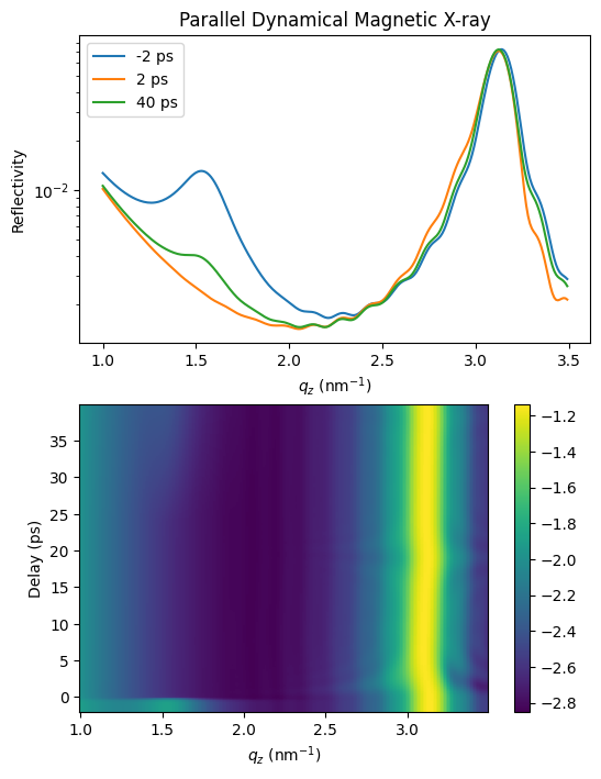
Parallel dynamical X-ray scattering

Parallelization is fundamentally implemented but needs further improvements. It works similar as with XrayDyn.

You need to install the udkm1Dsim with the parallel option which essentially add the Dask package to the requirements:

> pip install udkm1Dsim[parallel]

You can also install/add Dask manually, e.g. via pip:

> pip install dask

Please refer to the Dask documentation for more details on parallel computing in Python.

try:
    from dask.distributed import Client
    client = Client()
    R_seq_par, R_seq_phi_par, _, _ = dyn_mag.inhomogeneous_reflectivity(
        strain_map=strain_map,
        magnetization_map=magnetization_map,
        calc_type='parallel', dask_client=client
    )
    client.close()
except:
    pass

Calculating _inhomogeneous_reflectivity_ ...
Elapsed time for _inhomogeneous_reflectivity_: 818.527532 s

plt.figure(figsize=[6, 8])
plt.subplot(2, 1, 1)
plt.semilogy(dyn_mag.qz[0, :].to('1/nm'), R_seq_par[0, 0, :], label=np.round(delays[0]))
plt.semilogy(dyn_mag.qz[0, :].to('1/nm'), R_seq_par[40, 0, :], label=np.round(delays[40]))
plt.semilogy(dyn_mag.qz[0, :].to('1/nm'), R_seq_par[-1, 0, :], label=np.round(delays[-1]))

plt.xlabel('$q_z$ [nm$^{-1}$]')
plt.ylabel('Reflectivity')
plt.legend()
plt.title('Parallel Dynamical Magnetic X-ray')

plt.subplot(2, 1, 2)
plt.pcolormesh(dyn_mag.qz[0, :].to('1/nm').magnitude, delays.to('ps').magnitude,
               np.log10(R_seq_par[:, 0, :]), shading='auto')

plt.ylabel('Delay [ps]')
plt.xlabel('$q_z$ [nm$^{-1}$]')
plt.colorbar()
plt.show()