Data Fitting

Especially for light-scattering simulations, it is very common to also fit the simulations to some experimental data.

The udkm1Dsim toolbox is also able to do so using external fitting/minimizing packages such as scipy.optimize.minimize or lmfit.

In this example we first generate some experimental data by doing resonant magnetic scattering simulations for a given magnetization_map, which we resue from the M3TM model example. For the x-ray scattering, we will assume that the magnetic layer is made of Fe instead of CoNi.

In the fitting procedure, we will try to recover a simplified magnetization_map from the experimental data.

Setup

Do all necessary imports and settings.

import udkm1Dsim as ud
u = ud.u  # import the pint unit registry from udkm1Dsim
import scipy.constants as constants
import numpy as np
import matplotlib.pyplot as plt
%matplotlib inline
u.setup_matplotlib()  # use matplotlib with pint units
from tqdm.auto import trange

Structure

Refer to the structure-example for more details.

Fe = ud.Atom('Fe', mag_amplitude=1, mag_phi=90*u.deg, mag_gamma=90*u.deg,
                   atomic_form_factor_path='./Fe.cf')
Si = ud.Atom('Si')

prop_Fe = {}

layer_Fe = ud.AmorphousLayer('Fe', 'Fe amorphous', thickness=1*u.nm,
                              density=7874*u.kg/u.m**3, atom=Fe, **prop_Fe)

prop_Si = {}

layer_Si = ud.AmorphousLayer('Si', "Si amorphous", thickness=1*u.nm, density=2336*u.kg/u.m**3,
                             atom=Si, **prop_Si)

S = ud.Structure('Fe on Si')

S.add_sub_structure(layer_Fe, 20)
S.add_sub_structure(layer_Si, 50)

Generate Experimental Data

Magnetization Map

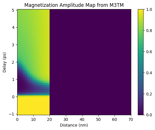
First we load the magnetization from the M3TM model example and convert it to a proper magnetization_map of amplitude and phi and gamma angles. Here we only adjust the amplitude and keep the orientation of the magnetization fixed out-of-plane.

m3tm_temp_map = np.load('m3tm_temp_map.npy')
# temporal grid is reduced by a factor of 10 to speed things up
m3tm_temp_map = m3tm_temp_map[0:-1:20, :, :]

magnetization_map = np.zeros_like(m3tm_temp_map)

for i in range(magnetization_map.shape[0]):
    # amplitude
    magnetization_map[i, :, 0] = m3tm_temp_map[i, :, 2]
    # phi
    magnetization_map[i, :, 1] = 0
    # gamma
    magnetization_map[i, :, 2] = 0


# compared to the M3TM example 
delays = np.linspace(-1, 5, magnetization_map.shape[0])*u.ps
# spatial grid
_, _, distances = S.get_distances_of_layers()

plt.figure()
plt.pcolormesh(distances.to('nm').magnitude, delays.to('ps').magnitude,
               magnetization_map[:, :, 0], shading='auto')
plt.title('Magnetization Amplitude Map from M3TM')
plt.ylabel('Delay (ps)')
plt.xlabel('Distance (nm)')
plt.colorbar()
plt.show()

Resonant Magnetic X-ray Scattering

dyn_mag = ud.XrayDynMag(S, True)
dyn_mag.disp_messages = True
dyn_mag.save_data = False

exp_energy = 708*u.eV
exp_qz = np.r_[1:3.5:0.01]/u.nm

dyn_mag.energy = exp_energy  # set the energy range
dyn_mag.qz = exp_qz  # qz range
dyn_mag.set_polarization(2, 0)

incoming polarizations set to: sigma
analyzer polarizations set to: unpolarized
incoming polarizations set to: circ -
analyzer polarizations set to: unpolarized

R, R_phi, _, _ = dyn_mag.inhomogeneous_reflectivity(
    magnetization_map=magnetization_map
)

Calculating _inhomogeneous_reflectivity_ ...

Elapsed time for _inhomogeneous_reflectivity_: 3.372442 s

# add some noise
noise_factor = 0.003
R_noisy = R*(1 + (np.random.random(R.shape)-0.5)*noise_factor)
R_phi_noisy = R_phi*(1 + (np.random.random(R.shape)-0.5)*noise_factor)

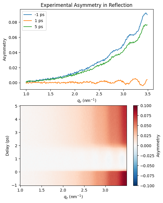
# calculate asymmetry
exp_asym = ((R_noisy-R_phi_noisy)/(R_noisy+R_phi_noisy))

plt.figure(figsize=[6, 8])
plt.subplot(2, 1, 1)
plt.plot(dyn_mag.qz[0, :].to('1/nm'), exp_asym[0, 0, :], label='{:.2~g}'.format(delays[0]))
plt.plot(dyn_mag.qz[0, :].to('1/nm'), exp_asym[20, 0, :], label='{:.2~g}'.format(delays[20]))
plt.plot(dyn_mag.qz[0, :].to('1/nm'), exp_asym[-1, 0, :], label='{:.2~g}'.format(delays[-1]))

plt.xlabel('$q_z$ (nm$^{-1}$)')
plt.ylabel('Asymmetry')
plt.legend()
plt.title('Experimental Asymmetry in Reflection')

plt.subplot(2, 1, 2)
plt.pcolormesh(dyn_mag.qz[0, :].to('1/nm').magnitude, delays.to('ps').magnitude,
               exp_asym[:, 0, :], shading='auto', vmin=-0.1, vmax=0.1, cmap='RdBu_r')

plt.ylabel('Delay (ps)')
plt.xlabel('$q_z$ (nm$^{-1}$)')
plt.colorbar(label='Asymmetry')
plt.show()

Fitting

For the fitting we will use the lmfit python package.

Attention

lmfit is not a dependency of the udkm1Dsim toolbox, so you need to install it yourself, e.g. by

pip install lmfit

or

conda install lmfit

In lmfit we build a fit Model by creating a function that best describes our experimental data. The function will depend on a set of parameters, which will eventually be optimized.

In our case, we will again calculate the x-ray asymmetry from a given sample structure. For the sake of simplicity, we just reuse the sample structure S from the data generation, see above. In reality, Layer parameters, such as thickness, density, or rhougness can be easily integrated in the fit procedure. Here, we will focus only on extracting a magnetization_map.

Again for simplicity, we will restrict the magnetization_map to follow a polynomial function in space $\( m(z) = a + b\,z + c\,z^2 \\ \)$ for every delay in time. This is of course only an educated guess and can be adjusted to your needs

Defining the Fit Function

def magnetization_profile(z, a, b, c):
    # simple polynomial function
    m = a + b*z + c*z**2
    return m

def xray_fitting_function(dyn_mag, a, b, c):
    dyn_mag.progress_bar = False
    dyn_mag.disp_messages = False
    L = dyn_mag.S.get_number_of_layers()
    # create a magnetization_map for a single delay
    # based on a, b, c
    magnetization_map = np.zeros([1, L, 3])
    z = np.arange(0, L)
    magnetization_map[0, :, 0] = magnetization_profile(z, a, b, c)
    R, R_phi, _, _ = dyn_mag.inhomogeneous_reflectivity(
        magnetization_map=magnetization_map
    )
    return ((R[0, :, :]-R_phi[0, :, :])/(R[0, :, :]+R_phi[0, :, :])).flatten()

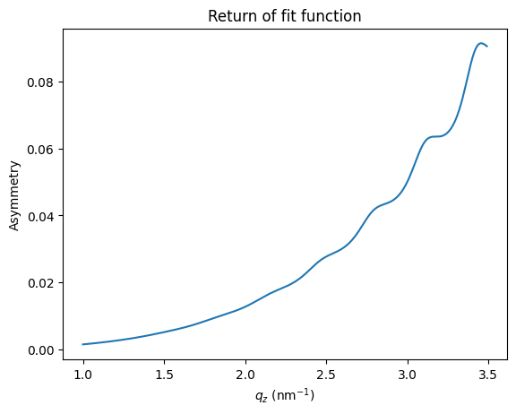
Let’s check what the function does for \(a=1\) which is a constant magnetization of 100%:

plt.figure()
plt.plot(exp_qz, xray_fitting_function(dyn_mag, 1, 0, 0))
plt.xlabel('$q_z$ (nm$^{-1}$)')
plt.ylabel('Asymmetry')
plt.title('Return of fit function')
plt.show()

Setup lmfit

import lmfit
# create a fitting model and tell lmfit which parameters are fixed/indepent
mod = lmfit.Model(xray_fitting_function, independent_vars=['dyn_mag'])

params = lmfit.Parameters()
params.add('a', value=1., vary=True)
params.add('b', value=0., vary=True)
params.add('c', value=0., vary=True)

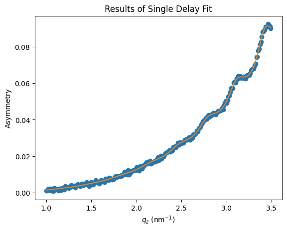
Running the fit for a single delay of the experimental data is just:

data2fit = exp_asym[0, 0, :]
res = mod.fit(data2fit, params=params, dyn_mag=dyn_mag)

plt.figure()
plt.plot(exp_qz, data2fit, 'o')
plt.plot(exp_qz, res.best_fit, '-')
plt.xlabel('$q_z$ (nm$^{-1}$)')
plt.ylabel('Asymmetry')
plt.title('Results of Single Delay Fit')
plt.show()

res.result

Fit Result

Fit Statistics

fitting method	leastsq
# function evals	17
# data points	250
# variables	3
chi-square	9.3014e-05
reduced chi-square	3.7658e-07
Akaike info crit.	-3695.05461
Bayesian info crit.	-3684.49023

Parameters

name	value	standard error	relative error	initial value	min	max	vary
a	0.99535911	0.00639063	(0.64%)	1.0	-inf	inf	True
b	-0.01115571	0.01421059	(127.38%)	0.0	-inf	inf	True
c	4.1956e-04	6.5632e-04	(156.43%)	0.0	-inf	inf	True

Correlations (unreported values are < 0.100)

Parameter1	Parameter 2	Correlation
b	c	-0.9944
a	b	+0.9851
a	c	-0.9759

That were obviously good starting values. Now lets run the fitting routine for all delays:

Fit Full Map

all_res = []
for i in trange(len(delays)):
    if i > 0:
        # use the results of the last fit
        # as starting values for the current one
        for key, par in params.items():
            params[key].value = all_res[i-1].best_values[key]

    data2fit = exp_asym[i, 0, :]
    all_res.append(mod.fit(data2fit, params=params, dyn_mag=dyn_mag))

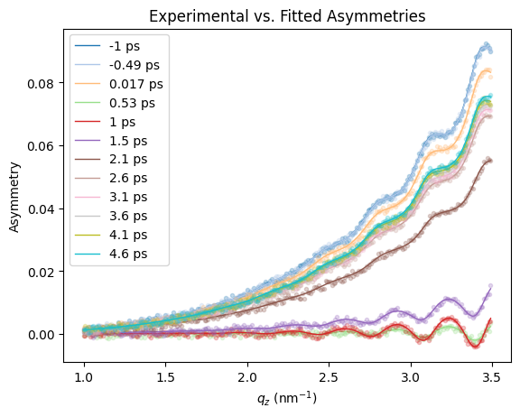
To be sure that the fitting worked out, we plot some of the experimental data together with the fit results for some selected delays:

colors = plt.get_cmap("tab20", 60)
plt.figure()
for i, r in enumerate(all_res):
    if np.mod(i, 5) == 0:
        data2fit = exp_asym[i, 0, :]
        plt.plot(exp_qz, data2fit, '.', color=colors(i), alpha=0.25)
        plt.plot(exp_qz, r.best_fit, '-', label='{:.2~g}'.format(delays[i]), color=colors(i), alpha=1, linewidth=1.)

plt.xlabel('$q_z$ (nm$^{-1}$)')
plt.ylabel('Asymmetry')
plt.title('Experimental vs. Fitted Asymmetries')
plt.legend()
plt.show()

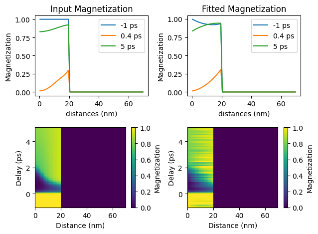
Plot the fitted magnetization_map in comparisson to the input map of the experimental data generation:

# assign fit results to magnetization_map
z = np.arange(0, len(distances))
fit_magnetization_map = np.zeros([len(delays), len(distances)])
for i, r in enumerate(all_res):
    # only assign first 20 elements for Fe layer
    fit_magnetization_map[i, 0:20] = magnetization_profile(
        z[0:20],
        r.best_values['a'],
        r.best_values['b'],
        r.best_values['c']
        )

plt.figure()
# input lineouts
plt.subplot(2, 2, 1)

plt.plot(distances.to('nm'), magnetization_map[0, :, 0], label='{:.1~g}'.format(delays[0]))
plt.plot(distances.to('nm'), magnetization_map[14, :, 0], label='{:.1~g}'.format(delays[14]))
plt.plot(distances.to('nm'), magnetization_map[-1, :, 0], label='{:.1~g}'.format(delays[-1]))
plt.xlabel('distances (nm)')
plt.ylabel('Magnetization')
plt.legend()
plt.title('Input Magnetization')

# fit results lineouts
plt.subplot(2, 2, 2)

plt.plot(distances.to('nm'), fit_magnetization_map[0, :], label='{:.1~g}'.format(delays[0]))
plt.plot(distances.to('nm'), fit_magnetization_map[14, :], label='{:.1~g}'.format(delays[14]))
plt.plot(distances.to('nm'), fit_magnetization_map[-1, :], label='{:.1~g}'.format(delays[-1]))
plt.xlabel('distances (nm)')
plt.ylabel('Magnetization')
plt.legend()
plt.title('Fitted Magnetization')

# input map
plt.subplot(2, 2, 3)

plt.pcolormesh(distances.to('nm').magnitude, delays.to('ps').magnitude,
               magnetization_map[:, :, 0], shading='auto', vmin=0, vmax=1)

plt.ylabel('Delay (ps)')
plt.xlabel('Distance (nm)')
plt.colorbar(label='Magnetization')

# fit results map
plt.subplot(2, 2, 4)

plt.pcolormesh(distances.to('nm'), delays.to('ps'),
               fit_magnetization_map[:, :], shading='auto', vmin=0, vmax=1)
plt.ylabel('Delay (ps)')
plt.xlabel('Distance (nm)')
plt.colorbar(label='Magnetization')

plt.tight_layout()
plt.show()

The fitting loop over different delays can be also easily parallelized, using e.g. dask.