XUV Polarimetry#
This example extends the previous one on Dynamical Magnetic X-ray Scattering by showcasing the ability to simulate with variable incoming and outcoing polarization in the XUV and soft-X-ray spectral range.
Added in version 2.4.0: Enable variable/elliptical polarization in XrayDynMag
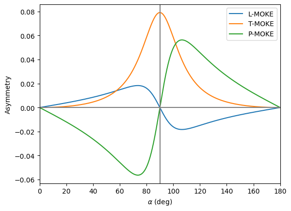
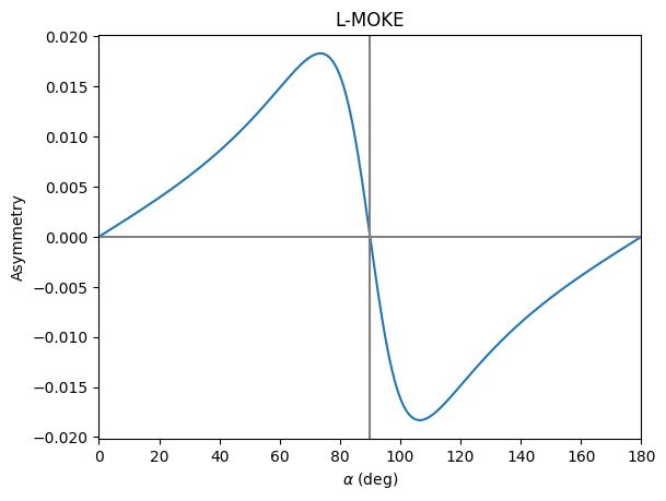
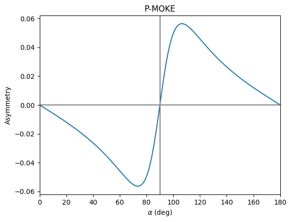
With that it is possible to extend the simulations beyond common geometries of XMCD and transversal MOKE (T-MOKE) to also probe in longitudinal and polar MOKE geometry, L-MOKE and P-MOKE, respectively.
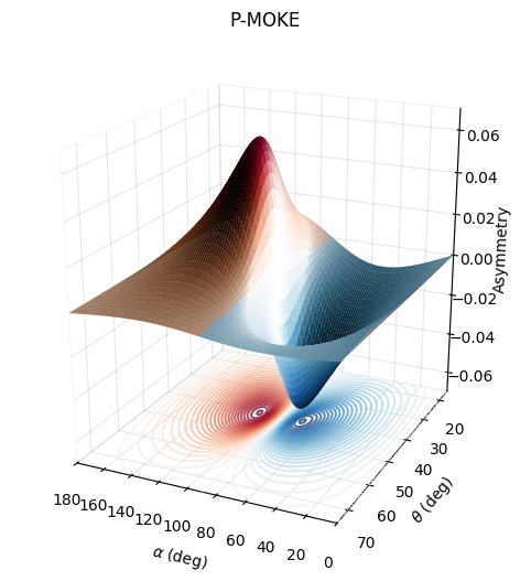
Since polarizing optics are hardly available/feasible in the XUV and soft-X-ray spectral range, L- and P-MOKE rely on the sample reflection itself close to the Brewster angle as polarization analyzer. Or in other words, the exact Brewster angle relies on the magnetization and polarization-dependent refractive index.
See also
Richter, J., et al., Spectroscopic probe of ultrafast magnetization dynamics in the extreme ultraviolet spectral range, Phys. Rev. B 111, 214423 (2025)
An overview of the different geometries are given in the following sketch form Richter, et al.:
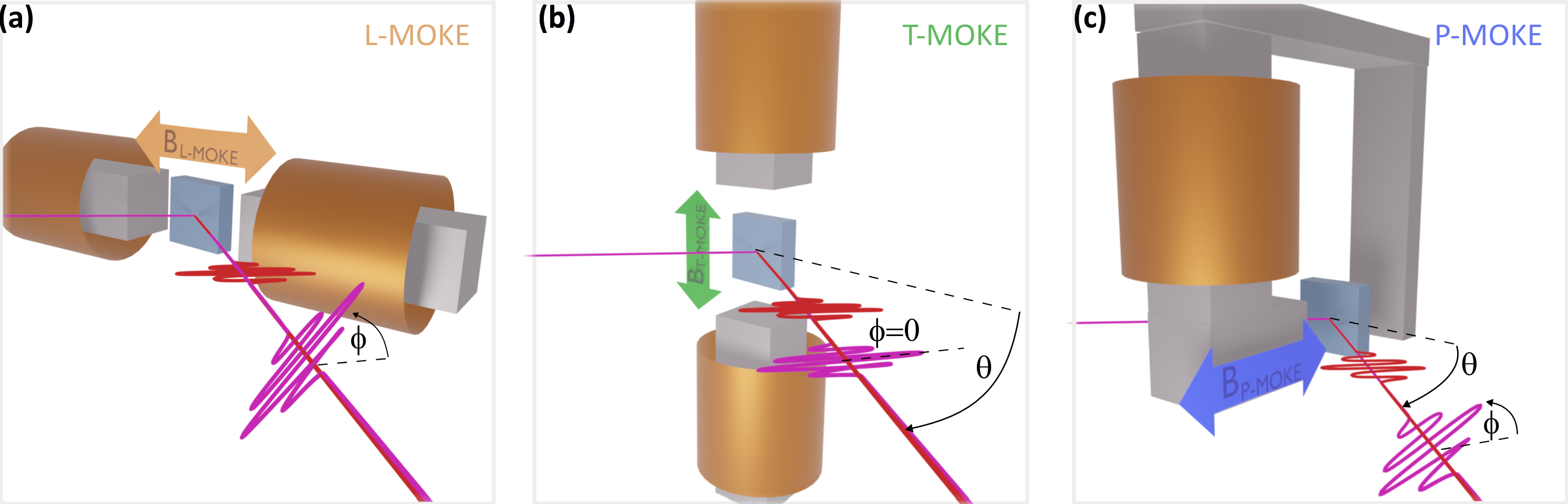
Note, that for L- and P-MOKE the linear polarization must be slightly tilted out of the scattering plane.
Attention
In the current example, the polarization angle is referred to as \(\alpha\) and NOT \(\phi\) as in the sketch from the paper in order to not confuse it with the polar coordinate of the magnetization as otherwise used in the udkm1Dsim toolbox, see User Guide for details. There is further 90° offset between both polarization angles.
The following table summarizes the experimental configurations:
(a) L-MOKE |
(b) T-MOKE |
(c) P-MOKE |
|
|---|---|---|---|
magnetization \(\gamma\) |
90° |
0° |
- |
magnetization \(\phi\) |
90° |
90° |
0° |
polarization \(\alpha\) |
\(\neq\) 90° |
\(=\) 90° |
\(\neq\) 90° |
Setup#
Do all necessary imports and settings.
import udkm1Dsim as ud
u = ud.u  # import the pint unit registry from udkm1Dsim
import numpy as np
import matplotlib.pyplot as plt
%matplotlib inline
u.setup_matplotlib()  # use matplotlib with pint units
Structure#
Refer to the structure example for more details.
In the XUV spectral range, the atomic form factors from the Henke tables are more suitable and can be selected by the keyword atomic_form_factor_source in the Atom constructor.
Ta = ud.Atom('Ta', atomic_form_factor_source='henke')
Ru = ud.Atom('Ru', atomic_form_factor_source='henke')

Si = ud.Atom('Si', atomic_form_factor_source='henke')
O = ud.Atom('O',  atomic_form_factor_source='henke')

SiO2  = ud.AtomMixed('SiO2')
SiO2.add_atom(Si, 0.33)
SiO2.add_atom(O, 0.67)
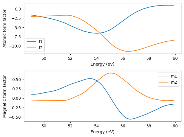
For the magnetic Fe atom experimental data for the charge and magnetic form factors is used.
See also
Willems, F., et al. Magneto-optical functions at the 3p resonances of Fe, Co, and Ni: Ab initio description and experiment, Phys. Rev. Lett. 122, 217202 (2019).
Fe = ud.Atom('Fe', mag_amplitude=1, mag_phi=90*u.deg, mag_gamma=180*u.deg,
             atomic_form_factor_path='./Fe_XUV.cf',
             magnetic_form_factor_path='./Fe_XUV.mf')
energies = np.r_[49:60:0.1]*u.eV

plt.figure()

plt.subplot(2,1,1)

plt.plot(energies, np.real(Fe.get_atomic_form_factor(energies)), label='f1')
plt.plot(energies, np.imag(Fe.get_atomic_form_factor(energies)), label='f2')

plt.legend()
plt.xlabel('Energy (eV)')
plt.ylabel('Atomic form factor')

plt.subplot(2,1,2)
plt.plot(energies, np.real(Fe.get_magnetic_form_factor(energies)), label='m1')
plt.plot(energies, np.imag(Fe.get_magnetic_form_factor(energies)), label='m2')

plt.legend()
plt.xlabel('Energy (eV)')
plt.ylabel('Magnetic form factor')

plt.tight_layout()
plt.show()
layer_Ta = ud.AmorphousLayer('Ta', 'Ta amorphous', 3*u.nm, 16650*u.kg/u.m**3, atom=Ta)
layer_Ru = ud.AmorphousLayer('Ru', 'Ru amorphous', 2*u.nm, 12370*u.kg/u.m**3, atom=Ru)
layer_SiO2 = ud.AmorphousLayer('SiO2', 'SiO2 amorphous',  100*u.nm, 2650*u.kg/u.m**3, atom=SiO2)
layer_Fe = ud.AmorphousLayer('Fe', 'Fe amorphous', 8*u.nm, 7874*u.kg/u.m**3, atom=Fe)
S = ud.Structure('Fe MOKE')

S.add_sub_structure(layer_Ru,1)
S.add_sub_structure(layer_Fe, 1)
S.add_sub_structure(layer_Ta, 1)
S.add_sub_structure(layer_SiO2, 1)
S.visualize()

Initialize dynamical magnetic X-ray simulations#
Please refer to the Dynamical Magnetic X-ray Scattering example for more details.
dyn_mag = ud.XrayDynMag(S, True)
dyn_mag.disp_messages = True
dyn_mag.save_data = False
incoming polarizations set to: sigma
analyzer polarizations set to: unpolarized
dyn_mag.energy = 54*u.eV
dyn_mag.theta = np.r_[45]*u.deg
Polarization settings#
In all following simulations the analyzer polarization is kept as unpolarized, which is equivalent to
dyn_mag.set_outgoing_polarization(0)
To enable variable/elliptical incoming polarization, the pol_in_state must be set to 5 in the set_incoming_polarization method.
Added in version 2.4.0: Enable variable/elliptical polarization in XrayDynMag
In this case a single tuple or list of tuples of the azimuth angle \(\alpha\) and the ellipticity \(e\) of the polarization can be input.
Note
alphas = np.r_[0:180:0.1]
dyn_mag.set_incoming_polarization(5, [(alpha*u.deg, 0) for alpha in alphas])
incoming polarizations set to: elliptical
T-MOKE#
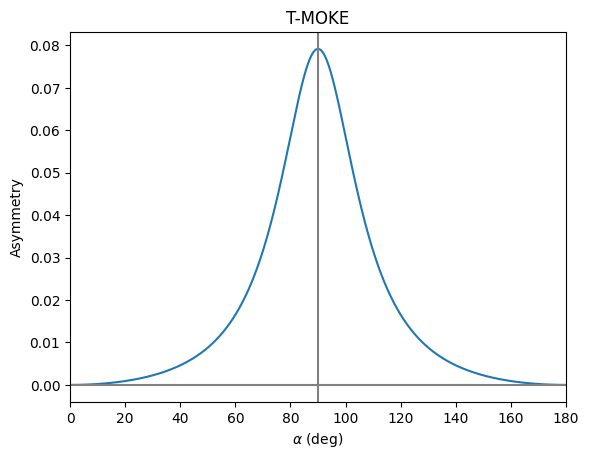
The current experimental configuration already corresponds to the well-known T-MOKE geometry.
Fe.mag_gamma = 180*u.deg  # s-pol
Fe.mag_phi = 90*u.deg  # in-plane

dyn_mag.theta = np.r_[45]*u.deg

R, R_phi, _, _ = dyn_mag.homogeneous_reflectivity()
asym_tmoke = ((R-R_phi)/(R+R_phi)).flatten()

plt.figure()
plt.plot(alphas, asym_tmoke)
plt.axvline(90, color='gray')
plt.axhline(0, color='gray')
plt.xlabel(r'$\alpha$ (deg)')
plt.ylabel('Asymmetry')
plt.xlim(0, 180)
plt.title('T-MOKE')
plt.show()
Calculating _homogeneous_reflectivity_ ...
Elapsed time for _homogeneous_reflectivity_: 0.036515 s
L-MOKE#
Fe.mag_gamma = 90*u.deg  # p-pol
Fe.mag_phi = 90*u.deg  # in-plane

dyn_mag.theta = np.r_[45]*u.deg

R, R_phi, _, _ = dyn_mag.homogeneous_reflectivity()
asym_lmoke = ((R-R_phi)/(R+R_phi)).flatten()

plt.figure()
plt.plot(alphas, asym_lmoke)
plt.axvline(90, color='gray')
plt.axhline(0, color='gray')
plt.xlabel(r'$\alpha$ (deg)')
plt.ylabel('Asymmetry')
plt.xlim(0, 180)
plt.title('L-MOKE')
plt.show()
Calculating _homogeneous_reflectivity_ ...
Elapsed time for _homogeneous_reflectivity_: 0.048053 s
P-MOKE#
Fe.mag_gamma = 0*u.deg  # any
Fe.mag_phi = 0*u.deg  # out-of-plane

dyn_mag.theta = np.r_[45]*u.deg

R, R_phi, _, _ = dyn_mag.homogeneous_reflectivity()
asym_pmoke = ((R-R_phi)/(R+R_phi)).flatten()

plt.figure()
plt.plot(alphas, asym_pmoke)
plt.axvline(90, color='gray')
plt.axhline(0, color='gray')
plt.xlabel(r'$\alpha$ (deg)')
plt.ylabel('Asymmetry')
plt.xlim(0, 180)
plt.title('P-MOKE')
plt.show()
Calculating _homogeneous_reflectivity_ ...
Elapsed time for _homogeneous_reflectivity_: 0.033113 s
dyn_mag.theta = np.r_[15:75:0.1]*u.deg
R, R_phi, _, _ = dyn_mag.homogeneous_reflectivity()
asym_pmoke_map = ((R-R_phi)/((R+R_phi)))

# 3D plotting
from matplotlib.colors import LightSource

fig = plt.figure(figsize=[8,6])
ax = fig.add_subplot(111, projection="3d")

X, Y = np.meshgrid(alphas, dyn_mag.theta[0, :].magnitude)
Z = asym_pmoke_map[0, :, :]

ls = LightSource(315, 10)
rgb = ls.shade(Z, cmap=plt.colormaps['RdBu_r'], vert_exag=10, blend_mode='hsv')

ax.plot_surface(X, Y, Z,
                linewidth=.1, antialiased=True, shade=False,
                facecolors=rgb, rstride=15, cstride=15)

ax.contour(X, Y, Z, zdir='z', offset=-0.07, cmap='RdBu_r', levels=50, alpha=0.75)

ax.set_ylabel(r'$\theta$ (deg)')
ax.set_xlabel(r'$\alpha$ (deg)')
ax.set_zlabel('Asymmetry')
ax.set_title('P-MOKE')

ax.set_xlim(0, 180)
ax.set_ylim(15, 75)
ax.set_zlim(-0.07, 0.07)

ax.view_init(elev=20., azim=115, roll=0, )
ax.set_proj_type('persp', focal_length=0.5)  # FOV = 157.4 deg
ax.set_box_aspect((3.5, 4, 4))
for axis in (ax.xaxis, ax.yaxis, ax.zaxis):
    axis.pane.fill = False
    axis._axinfo["grid"]["color"] = (0.1, 0.1, 0.1, 0.1)  # white grid lines
Calculating _homogeneous_reflectivity_ ...
Elapsed time for _homogeneous_reflectivity_: 0.177133 s
Comparison#
plt.figure()
plt.plot(alphas, asym_lmoke, label='L-MOKE')
plt.plot(alphas, asym_tmoke, label='T-MOKE')
plt.plot(alphas, asym_pmoke, label='P-MOKE')
plt.legend()
plt.axvline(90, color='gray')
plt.axhline(0, color='gray')
plt.xlabel(r'$\alpha$ (deg)')
plt.ylabel('Asymmetry')
plt.xlim(0, 180)
plt.show()