Heat#
In this example the laser-excitation of a sample Structure is shown.
It includes the actual absorption of the laser light as well as the transient temperature profile calculation.
Setup#
Do all necessary imports and settings.
import udkm1Dsim as ud
u = ud.u  # import the pint unit registry from udkm1Dsim
import scipy.constants as constants
import numpy as np
import matplotlib.pyplot as plt
%matplotlib inline
u.setup_matplotlib()  # use matplotlib with pint units
Structure#
Refer to the structure example for more details.
O = ud.Atom('O')
Ti = ud.Atom('Ti')
Sr = ud.Atom('Sr')
Ru = ud.Atom('Ru')
Pb = ud.Atom('Pb')
Zr = ud.Atom('Zr')
# c-axis lattice constants of the two layers
c_STO_sub = 3.905*u.angstrom
c_SRO = 3.94897*u.angstrom
# sound velocities [nm/ps] of the two layers
sv_SRO = 6.312*u.nm/u.ps
sv_STO = 7.800*u.nm/u.ps

# SRO layer
prop_SRO = {}
prop_SRO['a_axis'] = c_STO_sub  # aAxis
prop_SRO['b_axis'] = c_STO_sub  # bAxis
prop_SRO['deb_Wal_Fac'] = 0  # Debye-Waller factor
prop_SRO['sound_vel'] = sv_SRO  # sound velocity
prop_SRO['opt_ref_index'] = 2.44+4.32j
prop_SRO['therm_cond'] = 5.72*u.W/(u.m*u.K)  # heat conductivity
prop_SRO['lin_therm_exp'] = 1.03e-5  # linear thermal expansion
prop_SRO['heat_capacity'] = '455.2 + 0.112*T - 2.1935e6/T**2'  # [J/kg K]

SRO = ud.UnitCell('SRO', 'Strontium Ruthenate', c_SRO, **prop_SRO)
SRO.add_atom(O, 0)
SRO.add_atom(Sr, 0)
SRO.add_atom(O, 0.5)
SRO.add_atom(O, 0.5)
SRO.add_atom(Ru, 0.5)

# STO substrate
prop_STO_sub = {}
prop_STO_sub['a_axis'] = c_STO_sub  # aAxis
prop_STO_sub['b_axis'] = c_STO_sub  # bAxis
prop_STO_sub['deb_Wal_Fac'] = 0  # Debye-Waller factor
prop_STO_sub['sound_vel'] = sv_STO  # sound velocity
prop_STO_sub['opt_ref_index'] = 2.1+0j
prop_STO_sub['therm_cond'] = 12*u.W/(u.m*u.K)  # heat conductivity
prop_STO_sub['lin_therm_exp'] = 1e-5  # linear thermal expansion
prop_STO_sub['heat_capacity'] = '733.73 + 0.0248*T - 6.531e6/T**2'  #  [J/kg K]

STO_sub = ud.UnitCell('STOsub', 'Strontium Titanate Substrate',
                      c_STO_sub, **prop_STO_sub)
STO_sub.add_atom(O, 0)
STO_sub.add_atom(Sr, 0)
STO_sub.add_atom(O, 0.5)
STO_sub.add_atom(O, 0.5)
STO_sub.add_atom(Ti, 0.5)
S = ud.Structure('Single Layer')
S.add_sub_structure(SRO, 100)  # add 100 layers of SRO to sample
S.add_sub_structure(STO_sub, 200)  # add 200 layers of STO substrate
Initialize Heat#
The Heat class requires a Structure object and a boolean force_recalc in order overwrite previous simulation results.
These results are saved in the cache_dir when save_data is enabled.
Printing simulation messages can be en-/disabled using disp_messages and progress bars can using the boolean switch progress_bar.
h = ud.Heat(S, True)

h.save_data = False
h.disp_messages = True

print(h)
Heat simulation properties:

This is the current structure for the simulations:

Structure properties:

Name   : Single Layer
Thickness : 117.6 nm
Roughness : 0 nm
----
100 times Strontium Ruthenate: 39.49 nm
200 times Strontium Titanate Substrate: 78.1 nm
----
no substrate


Display properties:

================================  =======================================================
                       parameter  value
================================  =======================================================
                    force recalc  True
                 cache directory  ./
                display messages  True
                       save data  False
                    progress bar  True
              excitation fluence  [] mJ/cm²
                excitation delay  [0] ps
         excitation pulse length  [0] ps
           excitation wavelength  800 nm
                excitation theta  90 deg
         excitation polarization  p
excitation multilayer absorption  True
             excitation backside  False
                  heat diffusion  False
       interpolate at interfaces  11
                         backend  scipy
                       distances  no distance mesh is set for heat diffusion calculations
               top boundary type  isolator
            bottom boundary type  isolator
================================  =======================================================
Simple Excitation#
In order to calculate the temperature of the sample after quasi-instantaneous (delta) photoexcitation the excitation must be set with the following parameters:
fluencedelay_pumppulse_widthmultilayer_absorptionwavelengthpolarizationthetabackside
The angle of incidence theta does change the footprint of the excitation on the sample for any type excitation.
The wavelength and theta angle of the excitation are also relevant if multilayer_absorption = True, as well as the polarization (s or p).
Otherwise the Lambert_Beer-law is used and its absorption profile is independent of wavelength and theta.
With backside = True the excitation is calculated to happen from the backside of the sample structure.
Note: the fluence, delay_pump, and pulse_width must be given as array or list.
The simulation requires also a delay array as temporal grid as well as an initial temperature init_temp.
The later can be either a scalar which is then the constant temperature of the whole sample structure, or the initial temperature can be an array of temperatures for each single layer in the structure.
h.excitation = {'fluence': [5]*u.mJ/u.cm**2,
                'delay_pump':  [0]*u.ps,
                'pulse_width':  [0]*u.ps,
                'multilayer_absorption': True,
                'wavelength': 800*u.nm,
                'polarization': 'p',
                'theta': 45*u.deg,
                'backside': False}

# when calculating the laser absorption profile using Lamber-Beer-law
# the opt_pen_depth must be set manually or calculated from the refractive index
SRO.set_opt_pen_depth_from_ref_index(800*u.nm)
STO_sub.set_opt_pen_depth_from_ref_index(800*u.nm)

# temporal and spatial grid
delays = np.r_[-10:200:0.1]*u.ps
_, _, distances = S.get_distances_of_layers()
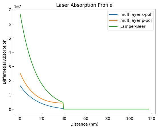
Laser Absorption Profile#
Here the difference in the spatial laser absorption profile is shown between the multilayer absorption algorithm and the Lambert-Beer law.
Note that Lambert-Beer does not include reflection of the incident light from the surface of the sample structure:
plt.figure()
h._excitation['polarization'] = 's'  # mind the "_" to directly set one entry of excitation
dAdz, _, _, _ = h.get_multilayers_absorption_profile()
plt.plot(distances.to('nm'), dAdz, label='multilayer s-pol')

h._excitation['polarization'] = 'p'
dAdz, _, _, _ = h.get_multilayers_absorption_profile()
plt.plot(distances.to('nm'), dAdz, label='multilayer p-pol')


dAdz = h.get_Lambert_Beer_absorption_profile()
plt.plot(distances.to('nm'), dAdz, label='Lamber-Beer')
plt.legend()
plt.xlabel('Distance (nm)')
plt.ylabel('Differnetial Absorption')
plt.title('Laser Absorption Profile')
plt.show()
Absorption profile is calculated by multilayer formalism with s-polarization.
Total reflectivity of 74.7 % and transmission of 3.2 %.
Absorption profile is calculated by multilayer formalism with p-polarization.
Total reflectivity of 56.1 % and transmission of 5.7 %.
Absorption profile is calculated by Lambert-Beer's law.
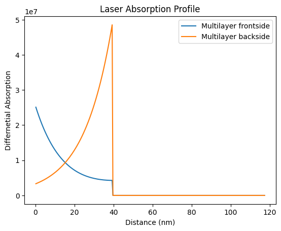
Backside Excitation#
The same calculation is repeated with the pump laser entering from the backside of the sample of the structure within the multilayer formalismus.
The clear difference in absorbed energy stems from the significantly different reflectivity of the pump light for front- or backside excitation due to better or worse refractive-index matching.
plt.figure()
dAdz, _, _, _ = h.get_multilayers_absorption_profile(backside=False)
plt.plot(distances.to('nm'), dAdz, label='Multilayer frontside')
dAdz, _, _, _ = h.get_multilayers_absorption_profile(backside=True)
plt.plot(distances.to('nm'), dAdz, label='Multilayer backside')
plt.legend()
plt.xlabel('Distance (nm)')
plt.ylabel('Differnetial Absorption')
plt.title('Laser Absorption Profile')
plt.show()
Absorption profile is calculated by multilayer formalism with p-polarization.
Total reflectivity of 56.1 % and transmission of 5.7 %.
Absorption profile is calculated by multilayer formalism with p-polarization.
Backside excitation is enabled.
Total reflectivity of 28.2 % and transmission of 71.8 %.
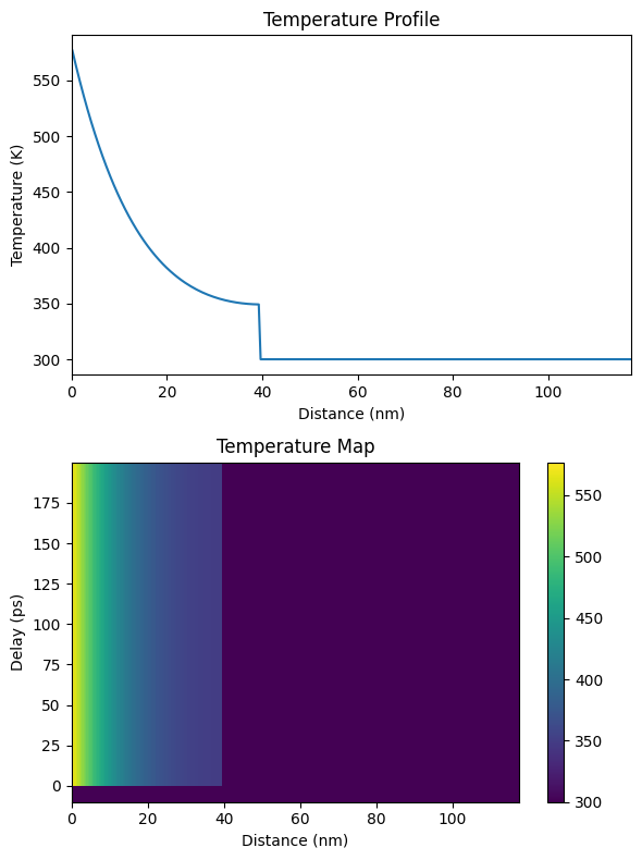
Temperature Map#
Calculating a tranient temperature map is only a one-line command:
temp_map, delta_temp = h.get_temp_map(delays, 300*u.K)
Surface incidence fluence scaled by factor 0.7071 due to incidence angle theta=45.00 deg
Absorption profile is calculated by multilayer formalism with p-polarization.
Total reflectivity of 56.1 % and transmission of 5.7 %.
Elapsed time for _temperature_after_delta_excitation_: 0.003962 s
Elapsed time for _temp_map_: 0.027396 s
plt.figure(figsize=[6, 8])
plt.subplot(2, 1, 1)
plt.plot(distances.to('nm').magnitude, temp_map[101, :])
plt.xlim([0, distances.to('nm').magnitude[-1]])
plt.xlabel('Distance (nm)')
plt.ylabel('Temperature (K)')
plt.title('Temperature Profile')

plt.subplot(2, 1, 2)
plt.pcolormesh(distances.to('nm').magnitude, delays.to('ps').magnitude, temp_map, shading='auto')
plt.colorbar()
plt.xlabel('Distance (nm)')
plt.ylabel('Delay (ps)')
plt.title('Temperature Map')

plt.tight_layout()
plt.show()
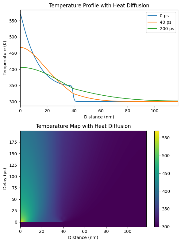
Heat Diffusion#
In order to enable heat diffusion the boolean switch heat_diffusion must be True.
It is also reasonable to define a finte pump pulse_width.
# enable heat diffusion
h.heat_diffusion = True
# set the boundary conditions
h.boundary_conditions = {'top_type': 'isolator', 'bottom_type': 'isolator'}
# change only the pulse duration
h.excitation = {'pulse_width':  [0.1]*u.ps}
# The resulting temperature profile is calculated in one line:
temp_map, delta_temp = h.get_temp_map(delays, 300*u.K)
Surface incidence fluence scaled by factor 0.7071 due to incidence angle theta=45.00 deg
Calculating _heat_diffusion_ for excitation 1:1 ...
Absorption profile is calculated by multilayer formalism with p-polarization.
Total reflectivity of 56.1 % and transmission of 5.7 %.
Elapsed time for _heat_diffusion_ with 1 excitation(s): 2.377584 s
Calculating _heat_diffusion_ without excitation...
Elapsed time for _heat_diffusion_: 3.700908 s
Elapsed time for _temp_map_: 6.140720 s
plt.figure(figsize=[6, 8])
plt.subplot(2, 1, 1)
plt.plot(distances.to('nm').magnitude, temp_map[101, :], label=np.round(delays[101]))
plt.plot(distances.to('nm').magnitude, temp_map[501, :], label=np.round(delays[501]))
plt.plot(distances.to('nm').magnitude, temp_map[-1, :], label=np.round(delays[-1]))
plt.xlim([0, distances.to('nm').magnitude[-1]])
plt.xlabel('Distance (nm)')
plt.ylabel('Temperature (K)')
plt.legend()
plt.title('Temperature Profile with Heat Diffusion')

plt.subplot(2, 1, 2)
plt.pcolormesh(distances.to('nm').magnitude, delays.to('ps').magnitude, temp_map, shading='auto')
plt.colorbar()
plt.xlabel('Distance (nm)')
plt.ylabel('Delay (ps)')
plt.title('Temperature Map with Heat Diffusion')

plt.tight_layout()
plt.show()
Heat Diffusion Parameters#
For heat diffusion simulations various parameters for the underlying pdepe solver can be altered.
By default, the backend is set to scipy but can be switched to matlab.
Currently, the is no obvious reason to choose MATLAB above SciPy.
Depending on the backend either the ode_options or ode_options_matlab can be configured and are directly handed to the actual solver.
Please refer to the documentation of the actual backend and solver and the API documentation for more details.
The speed but also the result of the heat diffusion simulation strongly depends on the spatial grid handed to the solver.
By default, one spatial grid point is used for every Layer (AmorphousLayer or UnitCell) in the Structure.
The resulting temp_map will also always be interpolated in this spatial grid which is equivalent to the distance vector returned by S.get_distances_of_layers().
As the solver for the heat diffusion usually suffers from large gradients, e.g. of thermal properties or initial temperatures, additional spatial grid points are added by default only for internal calculations. The number of additional points (should be an odd number, default is 11) is set by:
h.intp_at_interface = 11
The internally used spatial grid can be returned by:
dist_interp, original_indicies = S.interp_distance_at_interfaces(h.intp_at_interface)
The internal spatial grid can also be given by hand, e.g. to realize logarithmic steps for rather large Structures:
h.distances = np.linspace(0, distances.magnitude[-1], 100)*u.m
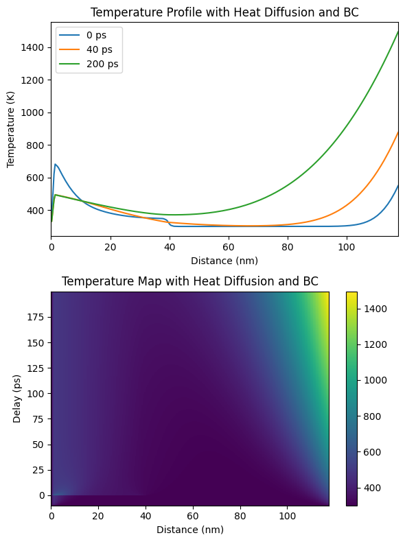
As already shown above, the heat diffusion simulation supports also an top and bottom boundary condition. The can have the types:
isolatortemperatureflux
For the later types also a value must be provides:
h.boundary_conditions = {'top_type': 'temperature', 'top_value': 500*u.K,
                         'bottom_type': 'flux', 'bottom_value': 5e11*u.W/u.m**2}

print(h)
Heat simulation properties:

This is the current structure for the simulations:

Structure properties:

Name   : Single Layer
Thickness : 117.6 nm
Roughness : 0 nm
----
100 times Strontium Ruthenate: 39.49 nm
200 times Strontium Titanate Substrate: 78.1 nm
----
no substrate


Display properties:

================================  =======================================================
                       parameter  value
================================  =======================================================
                    force recalc  True
                 cache directory  ./
                display messages  True
                       save data  False
                    progress bar  True
              excitation fluence  [5] mJ/cm²
                excitation delay  [0] ps
         excitation pulse length  [0.1] ps
           excitation wavelength  800 nm
                excitation theta  45 deg
         excitation polarization  p
excitation multilayer absorption  True
             excitation backside  False
                  heat diffusion  True
       interpolate at interfaces  11
                         backend  scipy
                       distances  a distance mesh is set for heat diffusion calculations.
               top boundary type  temperature
        top boundary temperature  500 K
            bottom boundary type  flux
            bottom boundary flux  5×10¹¹ W/m²
================================  =======================================================
# The resulting temperature profile is calculated in one line:
temp_map, delta_temp = h.get_temp_map(delays, 300*u.K)
Surface incidence fluence scaled by factor 0.7071 due to incidence angle theta=45.00 deg
Calculating _heat_diffusion_ without excitation...
Elapsed time for _heat_diffusion_: 0.515265 s
Calculating _heat_diffusion_ for excitation 1:1 ...
Absorption profile is calculated by multilayer formalism with p-polarization.
Total reflectivity of 56.1 % and transmission of 5.7 %.
Elapsed time for _heat_diffusion_ with 1 excitation(s): 0.455595 s
Calculating _heat_diffusion_ without excitation...
Elapsed time for _heat_diffusion_: 1.107343 s
Elapsed time for _temp_map_: 2.115993 s
plt.figure(figsize=[6, 8])
plt.subplot(2, 1, 1)
plt.plot(distances.to('nm').magnitude, temp_map[101, :], label=np.round(delays[101]))
plt.plot(distances.to('nm').magnitude, temp_map[501, :], label=np.round(delays[501]))
plt.plot(distances.to('nm').magnitude, temp_map[-1, :], label=np.round(delays[-1]))
plt.xlim([0, distances.to('nm').magnitude[-1]])
plt.xlabel('Distance (nm)')
plt.ylabel('Temperature (K)')
plt.legend()
plt.title('Temperature Profile with Heat Diffusion and BC')

plt.subplot(2, 1, 2)
plt.pcolormesh(distances.to('nm').magnitude, delays.to('ps').magnitude, temp_map, shading='auto')
plt.colorbar()
plt.xlabel('Distance (nm)')
plt.ylabel('Delay (ps)')
plt.title('Temperature Map with Heat Diffusion and BC')

plt.tight_layout()
plt.show()
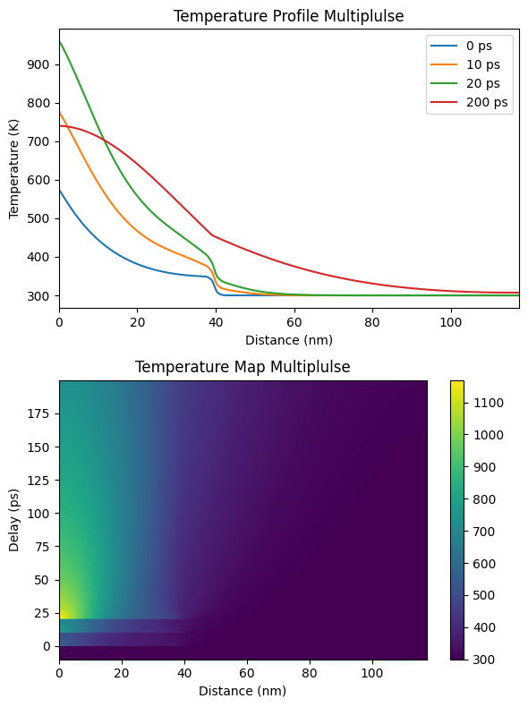
Multipulse Excitation#
As already stated above, also multiple pulses of variable fluence, pulse width and, delay are possible.
The heat diffusion simulation automatically splits the calculation in parts with and without excitation and adjusts the initial temporal step width according to the pulse width. Hence the solver does not miss any excitation pulses when adjusting its temporal step size.
The temporal laser pulse profile is always assumed to be Gaussian and the pulse width must be given as FWHM:
h.excitation = {'fluence': [5, 5, 5, 5]*u.mJ/u.cm**2,
                'delay_pump':  [0, 10, 20, 20.5]*u.ps,
                'pulse_width':  [0.1, 0.1, 0.1, 0.5]*u.ps,
                'multilayer_absorption': True,
                'wavelength': 800*u.nm,
                'theta': 45*u.deg,
                'backside': False
               }

h.boundary_conditions = {'top_type': 'isolator', 'bottom_type': 'isolator'}
# The resulting temperature profile is calculated in one line:
temp_map, delta_temp = h.get_temp_map(delays, 300*u.K)
Surface incidence fluence scaled by factor 0.7071 due to incidence angle theta=45.00 deg
Calculating _heat_diffusion_ for excitation 1:4 ...
Absorption profile is calculated by multilayer formalism with p-polarization.
Total reflectivity of 56.1 % and transmission of 5.7 %.
Elapsed time for _heat_diffusion_ with 1 excitation(s): 0.356385 s
Calculating _heat_diffusion_ without excitation...
Elapsed time for _heat_diffusion_: 0.413025 s
Calculating _heat_diffusion_ for excitation 2:4 ...
Absorption profile is calculated by multilayer formalism with p-polarization.
Total reflectivity of 56.1 % and transmission of 5.7 %.
Elapsed time for _heat_diffusion_ with 1 excitation(s): 0.179113 s
Calculating _heat_diffusion_ without excitation...
Elapsed time for _heat_diffusion_: 0.235615 s
Calculating _heat_diffusion_ for excitation 3-4:4...
Absorption profile is calculated by multilayer formalism with p-polarization.
Total reflectivity of 56.1 % and transmission of 5.7 %.
Elapsed time for _heat_diffusion_ with 2 excitation(s): 0.294813 s
Calculating _heat_diffusion_ without excitation...
Elapsed time for _heat_diffusion_: 0.310602 s
Elapsed time for _temp_map_: 1.877689 s
plt.figure(figsize=[6, 8])
plt.subplot(2, 1, 1)
plt.plot(distances.to('nm').magnitude, temp_map[101, :], label=np.round(delays[101]))
plt.plot(distances.to('nm').magnitude, temp_map[201, :], label=np.round(delays[201]))
plt.plot(distances.to('nm').magnitude, temp_map[301, :], label=np.round(delays[301]))
plt.plot(distances.to('nm').magnitude, temp_map[-1, :], label=np.round(delays[-1]))
plt.xlim([0, distances.to('nm').magnitude[-1]])
plt.xlabel('Distance (nm)')
plt.ylabel('Temperature (K)')
plt.legend()
plt.title('Temperature Profile Multiplulse')

plt.subplot(2, 1, 2)
plt.pcolormesh(distances.to('nm').magnitude, delays.to('ps').magnitude, temp_map, shading='auto')
plt.colorbar()
plt.xlabel('Distance (nm)')
plt.ylabel('Delay (ps)')
plt.title('Temperature Map Multiplulse')

plt.tight_layout()
plt.show()
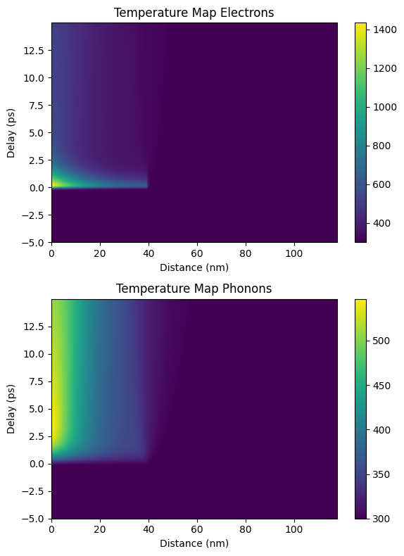
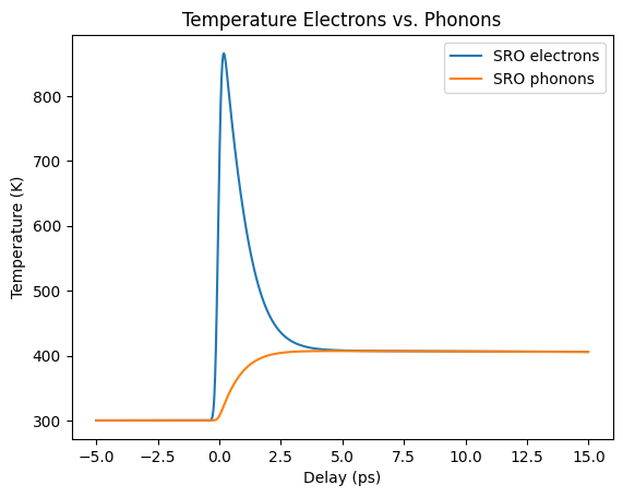
\(N\)-Temperature Model#
The heat diffusion is also capable of simulating an N-temperature model which is often applied to empirically simulate the energy flow between electrons, phonons, and spins. In order to run the NTM all thermo-elastic properties must be given as a list of N elements corresponding to different sub-systems. The actual external laser-excitation is always set to happen within the first sub-system, which is usually the electron-system.
In addition the sub_system_coupling must be provided in order to allow for energy-flow between the sub-systems.
sub_system_coupling is often set to a constant prefactor multiplied with the difference between the electronic and phononic temperatures, as in the example below.
For sufficiently high temperatures, this prefactor also depdends on temperature. See here for an overview.
In case the thermo-elastic parameters are provided as functions of the temperature \(T\), the sub_system_coupling requires the temperature T to be a vector of all sub-system-temperatures which can be accessed in the function string via the underscore-notation. The heat_capacity and lin_therm_exp instead require the temperature T to be a scalar of only the current sub-system-temperature. For the therm_cond both options are available.
# update the relevant thermo-elastic properties of the layers in the sample
# structure
SRO.therm_cond = [0,
                  5.72*u.W/(u.m*u.K)]
SRO.lin_therm_exp = [1.03e-5,
                     1.03e-5]
SRO.heat_capacity = ['0.112*T',
                     '455.2 - 2.1935e6/T**2']
SRO.sub_system_coupling = ['5e17*(T_1-T_0)',
                           '5e17*(T_0-T_1)']

STO_sub.therm_cond = [0,
                      12*u.W/(u.m*u.K)]
STO_sub.lin_therm_exp = [1e-5,
                         1e-5]
STO_sub.heat_capacity = ['0.0248*T',
                         '733.73 - 6.531e6/T**2']
STO_sub.sub_system_coupling = ['5e17*(T_1-T_0)',
                               '5e17*(T_0-T_1)']
Number of subsystems changed from 1 to 2.
Number of subsystems changed from 1 to 2.
As no new Structure is build, the num_sub_systems must be updated by hand.
Otherwise this happens automatically.
S.num_sub_systems = 2
Set the excitation conditions:
h.excitation = {'fluence': [5]*u.mJ/u.cm**2,
                'delay_pump':  [0]*u.ps,
                'pulse_width':  [0.25]*u.ps,
                'multilayer_absorption': True,
                'wavelength': 800*u.nm,
                'theta': 45*u.deg,
                'backside': False
               }

h.boundary_conditions = {'top_type': 'isolator', 'bottom_type': 'isolator'}

delays = np.r_[-5:15:0.01]*u.ps
# The resulting temperature profile is calculated in one line:
temp_map, delta_temp = h.get_temp_map(delays, 300*u.K)
Surface incidence fluence scaled by factor 0.7071 due to incidence angle theta=45.00 deg
Calculating _heat_diffusion_ for excitation 1:1 ...
Absorption profile is calculated by multilayer formalism with p-polarization.
Total reflectivity of 56.1 % and transmission of 5.7 %.
Elapsed time for _heat_diffusion_ with 1 excitation(s): 1.959294 s
Calculating _heat_diffusion_ without excitation...
Elapsed time for _heat_diffusion_: 1.204712 s
Elapsed time for _temp_map_: 3.205477 s
plt.figure(figsize=[6, 8])
plt.subplot(2, 1, 1)
plt.pcolormesh(distances.to('nm').magnitude, delays.to('ps').magnitude, temp_map[:, :, 0],
               shading='auto')
plt.colorbar()
plt.xlabel('Distance (nm)')
plt.ylabel('Delay (ps)')
plt.title('Temperature Map Electrons')

plt.subplot(2, 1, 2)
plt.pcolormesh(distances.to('nm').magnitude, delays.to('ps').magnitude, temp_map[:, :, 1],
               shading='auto')
plt.colorbar()
plt.xlabel('Distance (nm)')
plt.ylabel('Delay (ps)')
plt.title('Temperature Map Phonons')

plt.tight_layout()
plt.show()
plt.figure()
select = S.get_all_positions_per_unique_layer()['SRO']
plt.plot(delays.to('ps'), np.mean(temp_map[:, select, 0], 1), label='SRO electrons')
plt.plot(delays.to('ps'), np.mean(temp_map[:, select, 1], 1), label='SRO phonons')
plt.ylabel('Temperature (K)')
plt.xlabel('Delay (ps)')
plt.legend()
plt.title('Temperature Electrons vs. Phonons')
plt.show()
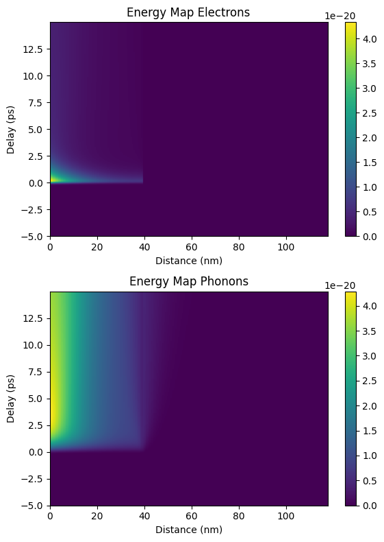
Energy map#
It is also possible to translate the temperature maps into energy maps and energy flux maps. The later is especially interesting for multi-subsystem simulations.
Added in version 2.4.0: Calculation of energy maps and energy flux maps from heat diffusion in Heat
energy_map = h.calc_energy_map(temp_map, 300*u.K)

plt.figure(figsize=[6, 8])
plt.subplot(2, 1, 1)
plt.pcolormesh(distances.to('nm').magnitude, delays.to('ps').magnitude, energy_map[:, :, 0],
               shading='auto')
plt.colorbar()
plt.xlabel('Distance (nm)')
plt.ylabel('Delay (ps)')
plt.title('Energy Map Electrons')

plt.subplot(2, 1, 2)
plt.pcolormesh(distances.to('nm').magnitude, delays.to('ps').magnitude, energy_map[:, :, 1],
               shading='auto')
plt.colorbar()
plt.xlabel('Distance (nm)')
plt.ylabel('Delay (ps)')
plt.title('Energy Map Phonons')

plt.tight_layout()
plt.show()
Elapsed time for _energy_map_: 0.515461 s
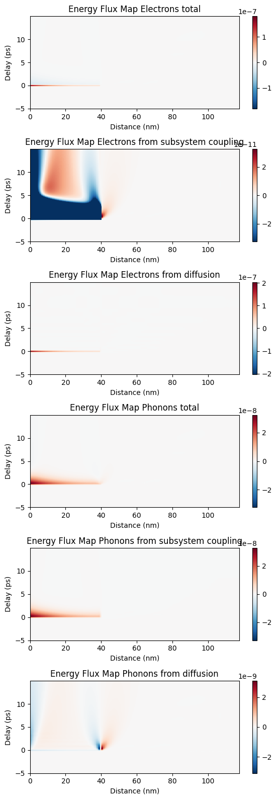
Energy Flux Map#
energy_flux_map = h.calc_energy_flux_map(temp_map, delta_temp, delays)

plt.figure(figsize=[6, 16])
plt.subplot(6, 1, 1)
flux = energy_flux_map[:, :, 0, 0]
plt.pcolormesh(distances.to('nm').magnitude, delays.to('ps').magnitude, flux,
               shading='auto', cmap='RdBu_r', vmin=-np.max(flux), vmax=np.max(flux))
plt.colorbar()
plt.xlabel('Distance (nm)')
plt.ylabel('Delay (ps)')
plt.title('Energy Flux Map Electrons total')

plt.subplot(6, 1, 2)
flux = energy_flux_map[:, :, 0, 1]
plt.pcolormesh(distances.to('nm').magnitude, delays.to('ps').magnitude, flux,
               shading='auto', cmap='RdBu_r', vmin=-np.max(flux), vmax=np.max(flux))
plt.colorbar()
plt.xlabel('Distance (nm)')
plt.ylabel('Delay (ps)')
plt.title('Energy Flux Map Electrons from subsystem coupling')

plt.subplot(6, 1, 3)
flux = energy_flux_map[:, :, 0, 2]
plt.pcolormesh(distances.to('nm').magnitude, delays.to('ps').magnitude, flux,
               shading='auto', cmap='RdBu_r', vmin=-np.max(flux), vmax=np.max(flux))
plt.colorbar()
plt.xlabel('Distance (nm)')
plt.ylabel('Delay (ps)')
plt.title('Energy Flux Map Electrons from diffusion')

plt.subplot(6, 1, 4)
flux = energy_flux_map[:, :, 1, 0]
plt.pcolormesh(distances.to('nm').magnitude, delays.to('ps').magnitude, flux,
               shading='auto', cmap='RdBu_r', vmin=-np.max(flux), vmax=np.max(flux))
plt.colorbar()
plt.xlabel('Distance (nm)')
plt.ylabel('Delay (ps)')
plt.title('Energy Flux Map Phonons total')

plt.subplot(6, 1, 5)
flux = energy_flux_map[:, :, 1, 1]
plt.pcolormesh(distances.to('nm').magnitude, delays.to('ps').magnitude, flux,
               shading='auto', cmap='RdBu_r', vmin=-np.max(flux), vmax=np.max(flux))
plt.colorbar()
plt.xlabel('Distance (nm)')
plt.ylabel('Delay (ps)')
plt.title('Energy Flux Map Phonons from subsystem coupling')

plt.subplot(6, 1, 6)
flux = energy_flux_map[:, :, 1, 2]
plt.pcolormesh(distances.to('nm').magnitude, delays.to('ps').magnitude, flux,
               shading='auto', cmap='RdBu_r', vmin=-np.max(flux), vmax=np.max(flux))
plt.colorbar()
plt.xlabel('Distance (nm)')
plt.ylabel('Delay (ps)')
plt.title('Energy Flux Map Phonons from diffusion')

plt.tight_layout()
plt.show()
Elapsed time for _energy_flux_map_: 1.568547 s