Microscopic 3-Temperature-Model#
Here we adapt the NTM from the heat example to allow for calculations of the magnetization within the microscopic 3-temperature-model.
Reference
Koopmans, B., Malinowski, G., Dalla Longa, F. et al.
Explaining the paradoxical diversity of ultrafast laser-induced demagnetization.
Nature Mater 9, 259–265 (2010).
We need to solve the following coupled differential equations:
We treat the temperature of the 3rd subsystem as magnetization \(m\).
For that we have to set its heat_capacity to \(1/\rho\) and thermal_conductivity to zero.
We put the complete right term of the last equation in the sub_system_coupling term for the 3rd subsystem.
Here, we need to rewrite the kotangens hyperbolicus in Python as
The values of the used parameters are not experimentally verified.
Setup#
Do all necessary imports and settings.
import udkm1Dsim as ud
u = ud.u  # import the pint unit registry from udkm1Dsim
import scipy.constants as constants
import numpy as np
import matplotlib.pyplot as plt
%matplotlib inline
u.setup_matplotlib()  # use matplotlib with pint units
Structure#
Refer to the structure example for more details.
Co = ud.Atom('Co')
Ni = ud.Atom('Ni')
CoNi = ud.AtomMixed('CoNi')
CoNi.add_atom(Co, 0.5)
CoNi.add_atom(Ni, 0.5)
Si = ud.Atom('Si')
prop_CoNi = {}
prop_CoNi['heat_capacity'] = ['0.1*T',
                              532*u.J/u.kg/u.K,
                              1/7000
                             ]
prop_CoNi['therm_cond'] = [20*u.W/(u.m*u.K),
                           80*u.W/(u.m*u.K),
                           0]

R = 25.3/1e-12
Tc = 1388
g = 4.0e18

prop_CoNi['sub_system_coupling'] = \
    ['-{:f}*(T_0-T_1)'.format(g),
     '{:f}*(T_0-T_1)'.format(g),
     '{0:f}*T_2*T_1/{1:f}*(1-T_2* (1 + 2/(exp(2*T_2*{1:f}/T_0) - 1) ))'.format(R, Tc)
    ]
prop_CoNi['lin_therm_exp'] = [0, 11.8e-6, 0]
prop_CoNi['sound_vel'] = 4.910*u.nm/u.ps
prop_CoNi['opt_ref_index'] = 2.9174+3.3545j

layer_CoNi = ud.AmorphousLayer('CoNi', 'CoNi amorphous', thickness=1*u.nm,
                               density=7000*u.kg/u.m**3, atom=CoNi, **prop_CoNi)
Number of subsystems changed from 1 to 3.
prop_Si = {}
prop_Si['heat_capacity'] = [100*u.J/u.kg/u.K, 603*u.J/u.kg/u.K, 1]
prop_Si['therm_cond'] = [0, 100*u.W/(u.m*u.K), 0]

prop_Si['sub_system_coupling'] = [0, 0, 0]

prop_Si['lin_therm_exp'] = [0, 2.6e-6, 0]
prop_Si['sound_vel'] = 8.433*u.nm/u.ps
prop_Si['opt_ref_index'] = 3.6941+0.0065435j

layer_Si = ud.AmorphousLayer('Si', "Si amorphous", thickness=1*u.nm, density=2336*u.kg/u.m**3,
                             atom=Si, **prop_Si)
Number of subsystems changed from 1 to 3.
S = ud.Structure('CoNi')

S.add_sub_structure(layer_CoNi, 20)
S.add_sub_structure(layer_Si, 50)
S.visualize()

Initialize Heat and the Excitation#
h = ud.Heat(S, True)

h.save_data = False
h.disp_messages = True
h.excitation = {'fluence': [30]*u.mJ/u.cm**2,
                'delay_pump':  [0]*u.ps,
                'pulse_width':  [0.05]*u.ps,
                'multilayer_absorption': True,
                'wavelength': 800*u.nm,
                'theta': 45*u.deg}
# temporal and spatial grid
delays = np.r_[-1:5:0.005]*u.ps
_, _, distances = S.get_distances_of_layers()
Calculate Heat Diffusion#
The init_temp sets the magnetization in the 3rd subsystem to 1 for CoNi and 0 for Si.
# enable heat diffusion
h.heat_diffusion = True
# set the boundary conditions
h.boundary_conditions = {'top_type': 'isolator', 'bottom_type': 'isolator'}
# The resulting temperature profile is calculated in one line:

init_temp = np.ones([S.get_number_of_layers(), 3])
init_temp[:, 0] = 300
init_temp[:, 1] = 300
init_temp[20:, 2] = 0

temp_map, delta_temp = h.get_temp_map(delays, init_temp)
Surface incidence fluence scaled by factor 0.7071 due to incidence angle theta=45.00 deg
Calculating _heat_diffusion_ without excitation...
Elapsed time for _heat_diffusion_: 1.453138 s
Calculating _heat_diffusion_ for excitation 1:1 ...
Absorption profile is calculated by multilayer formalism with p-polarization.
Total reflectivity of 42.4 % and transmission of 28.4 %.
Elapsed time for _heat_diffusion_ with 1 excitation(s): 1.421014 s
Calculating _heat_diffusion_ without excitation...
Elapsed time for _heat_diffusion_: 4.915753 s
Elapsed time for _temp_map_: 7.830717 s
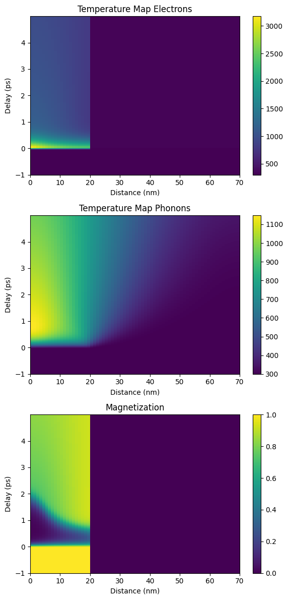
plt.figure(figsize=[6, 12])
plt.subplot(3, 1, 1)
plt.pcolormesh(distances.to('nm').magnitude, delays.to('ps').magnitude, temp_map[:, :, 0],
               shading='auto')
plt.colorbar()
plt.xlabel('Distance (nm)')
plt.ylabel('Delay (ps)')
plt.title('Temperature Map Electrons')

plt.subplot(3, 1, 2)
plt.pcolormesh(distances.to('nm').magnitude, delays.to('ps').magnitude, temp_map[:, :, 1],
               shading='auto')
plt.colorbar()
plt.xlabel('Distance (nm)')
plt.ylabel('Delay (ps)')
plt.title('Temperature Map Phonons')

plt.subplot(3, 1, 3)
plt.pcolormesh(distances.to('nm').magnitude, delays.to('ps').magnitude,
               temp_map[:, :, 2], shading='auto')
plt.colorbar()
plt.xlabel('Distance (nm)')
plt.ylabel('Delay (ps)')
plt.title('Magnetization')

plt.tight_layout()
plt.show()
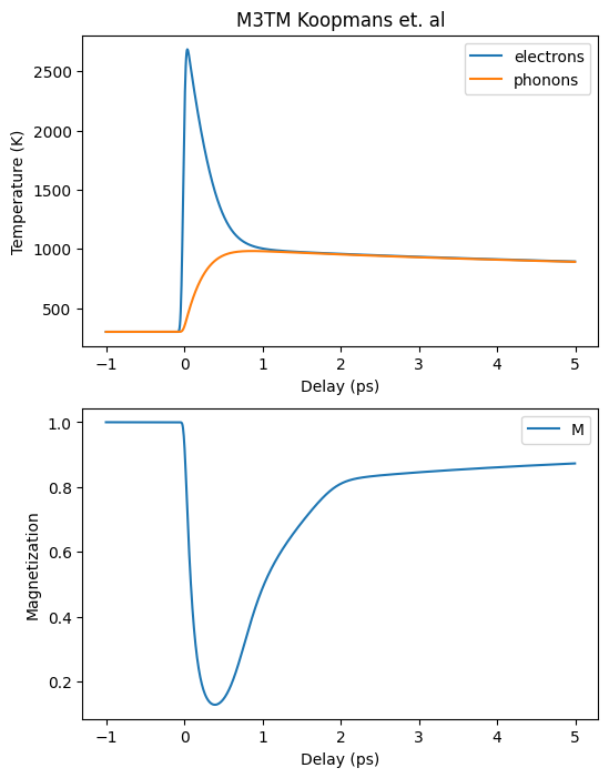
plt.figure(figsize=[6, 8])
plt.subplot(2, 1, 1)
select = S.get_all_positions_per_unique_layer()['CoNi']
plt.plot(delays.to('ps'), np.mean(temp_map[:, select, 0], 1), label='electrons')
plt.plot(delays.to('ps'), np.mean(temp_map[:, select, 1], 1), label='phonons')
plt.ylabel('Temperature (K)')
plt.xlabel('Delay (ps)')
plt.legend()
plt.title('M3TM Koopmans et. al')

plt.subplot(2, 1, 2)

plt.plot(delays.to('ps'), np.mean(temp_map[:, select, 2], 1), label='M')
plt.ylabel('Magnetization')
plt.xlabel('Delay (ps)')
plt.legend()
plt.show()