3-Temperature-Model with Criticality#

Here, the NTM from the excitation & NTM example is extended by a third subsystems for spins.
Reference [4]
D. Khusyainov, R. Liefferink, et al., Time-resolved magnetic force microscopy of all-optical magnetization switching APL Mater. 14, 061109 (2026)
This leads to the following system of coupled differential equations:
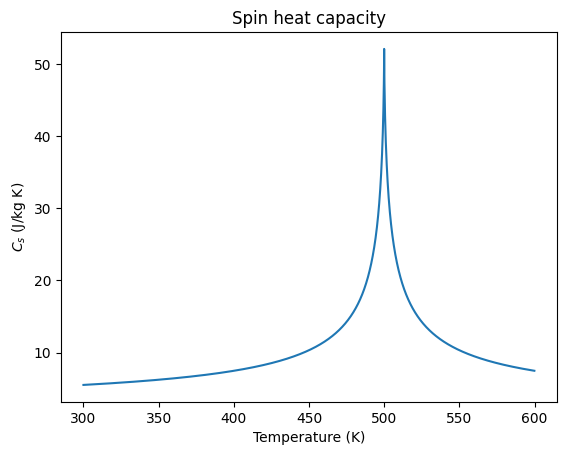
Moreover, to model critical behaviour of the spin heat capacity \(C_s(T)\) close to the Curie temperature \(T_C\), a phenomenological critical anomaly is of \(C_s(T)\) is introduced by:
The laser excitation is also modelled by \(i\) different laser pulse of variable delay, pulse width, and fluence.
Important
As in Khusyainov et al. [4] the example is simplified by neglecting thermal diffusion and following an effective-medium approach for the metallic Co and Pt layers.
A full simulation including thermal conductivity is easily possible with the udkm1Dsim, but would require the careful determination of a large number of sub-system-dependent material parameters.
Setup#
Do all necessary imports and settings.
try:
    import udkm1Dsim as ud
except ImportError:
    %pip install udkm1Dsim
    import udkm1Dsim as ud

u = ud.u  # import the pint unit registry from udkm1Dsim
import numpy as np
import matplotlib.pyplot as plt
%matplotlib inline
u.setup_matplotlib()  # use matplotlib with pint units
Structure#
Refer to the structure example for more details.
Co = ud.Atom('Co')
Pt = ud.Atom('Pt')
Mg = ud.Atom('Mg')
O = ud.Atom('O')
Ta = ud.Atom('Ta')
Si = ud.Atom('Si')

SiO2 = ud.AtomMixed('SiO2')
SiO2.add_atom(Si, 0.33)
SiO2.add_atom(O, 0.67)

MgO = ud.AtomMixed('MgO')
MgO.add_atom(Mg, 0.5)
MgO.add_atom(O, 0.5)
Hint
Some parameters from Khusyainov et al. [4] are volume-specific while the udkm1Dsim toolbox requires mass-specific parameters.
density_effective = (8900*u.kg/u.m**3 + 10*21000*u.kg/u.m**3)/11

gamma = 2.6e2/density_effective.magnitude  # in J/kg/K²
C_s0 = 4e4/density_effective.magnitude  # in J/kg/K
zeta = 24.9
alpha = 0.7
T_c = 500
Delta = 5  # in K
G_el = 1.9e18  # in W/m³
G_es = 2.4e17  # in W/m³
G_sl = 3.0e15  # in W/m³

prop_Co = {}
prop_Co['heat_capacity'] = [f'{gamma:f}*T',
                            f'(2.98e6 + 1.5e3*(T-300))/{density_effective.magnitude:f}',
                            f'{C_s0:f}*(1+{zeta:f}/(1+abs((T-{T_c:f})/{Delta:f})**{alpha:f}))'
                            ]

# only allow for electronic conduction to equilibrate Co and Pt
prop_Co['therm_cond'] = [1000, 0, 0]

prop_Co['sub_system_coupling'] = \
    [f'-{G_el:f}*(T_0-T_1)-{G_es:f}*(T_0-T_2)',
     f'-{G_el:f}*(T_1-T_0)-{G_sl:f}*(T_1-T_2)',
     f'-{G_es:f}*(T_2-T_0)-{G_sl:f}*(T_2-T_1)',
     ]
prop_Co['lin_therm_exp'] = [0, 0, 0]
prop_Co['opt_ref_index'] = 2.5+4.8j

layer_Co = ud.AmorphousLayer('Co', 'Co layer', thickness=0.1*u.nm,
                             density=density_effective, atom=Co, **prop_Co)
Number of subsystems changed from 1 to 3.
/home/schick/Programming/git/udkm1Dsim/udkm1Dsim/structures/layers.py:499: UserWarning:
The sympy integration of the heat capacity did not work. It is only required for

    Heat.get_temperature_after_delta_excitation()

You can set its analytical anti-derivative manually as a str representing the correct function of temperature T by typing

    layer.int_heat_capacity = 'c(T)'

where layer is the name of the layer object.

  warnings.warn('\nThe sympy integration of the heat capacity did not work. '
Important
The UserWarning above is not relevant for this example when calculating heat diffusion with a finite pulse duration.
prop_Pt = {}
prop_Pt['heat_capacity'] = prop_Co['heat_capacity']
prop_Pt['therm_cond'] = prop_Co['therm_cond']
prop_Pt['sub_system_coupling'] = prop_Co['sub_system_coupling']
prop_Pt['lin_therm_exp'] = [0, 0, 0]
prop_Pt['opt_ref_index'] = 2.7254+6.1280j  # A. Tselin, et al., Phys. Rev. B 110, 195130 (2024)

layer_Pt = ud.AmorphousLayer('Pt', 'Pt layer', 0.1*u.nm, density_effective, atom=Pt, **prop_Pt)
Number of subsystems changed from 1 to 3.
prop_Ta = {}
prop_Ta['heat_capacity'] = [40*u.J/u.kg/u.K, 100*u.J/u.kg/u.K, 1e-6]
prop_Ta['therm_cond'] = [0, 0, 0]
prop_Ta['sub_system_coupling'] = ['5e17*(T_1-T_0)',
                                  '5e17*(T_0-T_1)',
                                  0
                                  ]
prop_Ta['lin_therm_exp'] = [0, 0, 0]
prop_Ta['opt_ref_index'] = 1.111+3.4796j

layer_Ta = ud.AmorphousLayer('Ta', 'Ta layer', thickness=0.1*u.nm, density=16650*u.kg/u.m**3,
                             atom=Ta, **prop_Ta)
Number of subsystems changed from 1 to 3.
prop_Al = {}
prop_Al['heat_capacity'] = [200*u.J/u.kg/u.K, 700*u.J/u.kg/u.K, 1e-6]
prop_Al['therm_cond'] = [0, 0, 0]
prop_Al['sub_system_coupling'] = ['5e17*(T_1-T_0)',
                                  '5e17*(T_0-T_1)',
                                  0]
prop_Al['lin_therm_exp'] = [0, 0, 0]
prop_Al['opt_ref_index'] = 2.767+8.354j

layer_Al = ud.AmorphousLayer('Al', 'Al layer', thickness=0.1*u.nm, density=2700*u.kg/u.m**3,
                             atom=SiO2, **prop_Al)
Number of subsystems changed from 1 to 3.
prop_MgO = {}
prop_MgO['heat_capacity'] = [1e-6, 923*u.J/u.kg/u.K, 1e-6]
prop_MgO['therm_cond'] = [0, 0, 0]
prop_MgO['sub_system_coupling'] = [0, 0, 0]
prop_MgO['lin_therm_exp'] = [0, 0, 0]
prop_MgO['opt_ref_index'] = 1.72+0.0j

layer_MgO = ud.AmorphousLayer('MgO', 'MgO laser', thickness=0.1*u.nm, density=3580*u.kg/u.m**3,
                              atom=SiO2, **prop_MgO)
Number of subsystems changed from 1 to 3.
prop_glass = {}
prop_glass['heat_capacity'] = [1e-6, 700*u.J/u.kg/u.K, 1e-6]
prop_glass['therm_cond'] = [0, 0, 0]
prop_glass['sub_system_coupling'] = [0, 0, 0]
prop_glass['lin_therm_exp'] = [0, 0, 0]
prop_glass['opt_ref_index'] = 3.6941+0.0

layer_glass = ud.AmorphousLayer('glass', 'glass laser', thickness=1*u.nm, density=2650*u.kg/u.m**3,
                                atom=SiO2, **prop_glass)
Number of subsystems changed from 1 to 3.
S = ud.Structure('Sample')

S.add_sub_structure(layer_Ta, 10)
S.add_sub_structure(layer_MgO, 20)
S.add_sub_structure(layer_Pt, 30)
S.add_sub_structure(layer_Co, 6)
S.add_sub_structure(layer_Pt, 30)
S.add_sub_structure(layer_Ta, 40)
S.add_sub_structure(layer_glass, 10)
S.visualize()

Initialize Heat and the Excitation#
h = ud.Heat(S, True)

h.save_data = False
h.disp_messages = True

# enable heat diffusion
h.heat_diffusion = True
# set the boundary conditions
h.boundary_conditions = {'top_type': 'isolator', 'bottom_type': 'isolator'}
# spatial grid
_, _, distances = S.get_distances_of_layers()
# select only Co and Pt layers for plotting
select = np.concat((S.get_all_positions_per_unique_layer()['Co'],
                    S.get_all_positions_per_unique_layer()['Pt']))
delays = np.r_[-2.5:10:0.01]*u.ps

fluence = 3.5  # in mJ/cm²
Criticallity of Spin Heat Capacity#
temps = np.r_[300:600:0.1]

plt.figure()
plt.plot(temps, layer_Co.heat_capacity[2](temps))
plt.xlabel('Temperature (K)')
plt.ylabel('$C_s$ (J/kg K)')
plt.title('Spin heat capacity')
plt.show()
Absorption profile#
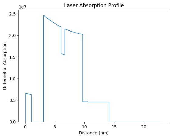
plt.figure()
dAdz, _, _, _ = h.get_multilayers_absorption_profile()
plt.stairs(dAdz[:-1], distances.to('nm'))
plt.xlabel('Distance (nm)')
plt.ylabel('Differnetial Absorption')
plt.title('Laser Absorption Profile')
plt.show()
Absorption profile is calculated by multilayer formalism with p-polarization.
Total reflectivity of 55.5 % and transmission of 27.9 %.
Single-Pulse Excitation#
100-fs-Pulse#
h.excitation = {'fluence': [fluence]*u.mJ/u.cm**2,
                'delay_pump':  [0]*u.ps,
                'pulse_width':  [0.1/2.355]*u.ps,  # from FWHM to sigma
                'multilayer_absorption': True,
                'wavelength': 800*u.nm,
                'theta': 90*u.deg}

temp_map_100fs, delta_temp_100fs = h.get_temp_map(delays, 300)
Surface incidence fluence scaled by factor 1.0000 due to incidence angle theta=90.00 deg
Calculating _heat_diffusion_ for excitation 1:1 ...
Absorption profile is calculated by multilayer formalism with p-polarization.
Total reflectivity of 55.5 % and transmission of 27.9 %.
Elapsed time for _heat_diffusion_ with 1 excitation(s): 17.187902 s
Calculating _heat_diffusion_ without excitation...
Elapsed time for _heat_diffusion_: 30.893136 s
Elapsed time for _temp_map_: 48.174044 s
3-ps-Pulse#
h.excitation = {'fluence': [fluence]*u.mJ/u.cm**2,
                'delay_pump':  [0]*u.ps,
                'pulse_width':  [3.0/2.355]*u.ps,  # from FWHM to sigma
                'multilayer_absorption': True,
                'wavelength': 800*u.nm,
                'theta': 90*u.deg}

temp_map_3ps, delta_temp_3ps = h.get_temp_map(delays, 300)
Surface incidence fluence scaled by factor 1.0000 due to incidence angle theta=90.00 deg
Calculating _heat_diffusion_ for excitation 1:1 ...
Absorption profile is calculated by multilayer formalism with p-polarization.
Total reflectivity of 55.5 % and transmission of 27.9 %.
Elapsed time for _heat_diffusion_ with 1 excitation(s): 32.941442 s
Calculating _heat_diffusion_ without excitation...
Elapsed time for _heat_diffusion_: 6.210651 s
Elapsed time for _temp_map_: 39.277871 s
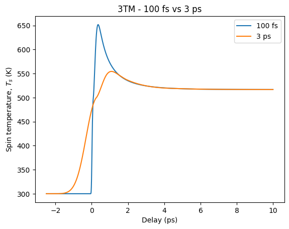
Comparison of Spin temperatures#
plt.figure()
plt.plot(delays.to('ps'), np.mean(temp_map_100fs[:, select, 2], 1), label='100 fs')
plt.plot(delays.to('ps'), np.mean(temp_map_3ps[:, select, 2], 1), label='3 ps')
plt.ylabel('Spin temperature, $T_s$ (K)')
plt.xlabel('Delay (ps)')
plt.legend()
plt.title('3TM - 100 fs vs 3 ps')
plt.show()
Double Pulse Excitation#
Hint
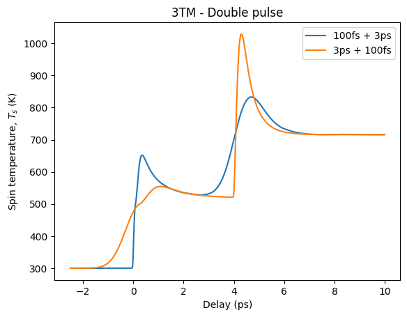
Multipluse excitation is readily available by the providing lists of fluence, delay_pump, and pulse_width of the excitation dictionary.
100 fs + 3 ps#
h.excitation = {'fluence': [fluence, fluence]*u.mJ/u.cm**2,
                'delay_pump':  [0, 4]*u.ps,
                'pulse_width':  [0.1, 3]*u.ps/2.355,
                'multilayer_absorption': True,
                'wavelength': 800*u.nm,
                'theta': 90*u.deg}

temp_map_100fs_3ps, delta_temp_100fs_3ps = h.get_temp_map(delays, 300)
Surface incidence fluence scaled by factor 1.0000 due to incidence angle theta=90.00 deg
Calculating _heat_diffusion_ for excitation 1:2 ...
Absorption profile is calculated by multilayer formalism with p-polarization.
Total reflectivity of 55.5 % and transmission of 27.9 %.
Elapsed time for _heat_diffusion_ with 1 excitation(s): 10.288944 s
Calculating _heat_diffusion_ without excitation...
Elapsed time for _heat_diffusion_: 24.157430 s
Calculating _heat_diffusion_ for excitation 2:2 ...
Absorption profile is calculated by multilayer formalism with p-polarization.
Total reflectivity of 55.5 % and transmission of 27.9 %.
Elapsed time for _heat_diffusion_ with 1 excitation(s): 25.755992 s
Calculating _heat_diffusion_ without excitation...
Elapsed time for _heat_diffusion_: 3.667309 s
Elapsed time for _temp_map_: 64.017149 s
3 ps + 100 fs#
h.excitation = {'fluence': [fluence, fluence]*u.mJ/u.cm**2,
                'delay_pump':  [0, 4]*u.ps,
                'pulse_width':  [3, 0.1]*u.ps/2.355,
                'multilayer_absorption': True,
                'wavelength': 800*u.nm,
                'theta': 90*u.deg}

temp_map_3ps_100fs, delta_temp_3ps_100fs = h.get_temp_map(delays, 300)
Surface incidence fluence scaled by factor 1.0000 due to incidence angle theta=90.00 deg
Calculating _heat_diffusion_ for excitation 1:2 ...
Absorption profile is calculated by multilayer formalism with p-polarization.
Total reflectivity of 55.5 % and transmission of 27.9 %.
Elapsed time for _heat_diffusion_ with 1 excitation(s): 28.563763 s
Calculating _heat_diffusion_ without excitation...
Elapsed time for _heat_diffusion_: 1.728633 s
Calculating _heat_diffusion_ for excitation 2:2 ...
Absorption profile is calculated by multilayer formalism with p-polarization.
Total reflectivity of 55.5 % and transmission of 27.9 %.
Elapsed time for _heat_diffusion_ with 1 excitation(s): 8.062905 s
Calculating _heat_diffusion_ without excitation...
Elapsed time for _heat_diffusion_: 31.274183 s
Elapsed time for _temp_map_: 69.829167 s
Comparison#
plt.figure()
plt.plot(delays.to('ps'), np.mean(temp_map_100fs_3ps[:, select, 2], 1), label='100fs + 3ps')
plt.plot(delays.to('ps'), np.mean(temp_map_3ps_100fs[:, select, 2], 1), label='3ps + 100fs')
plt.ylabel('Spin temperature, $T_s$ (K)')
plt.xlabel('Delay (ps)')
plt.legend()
plt.title('3TM - Double pulse')
plt.show()
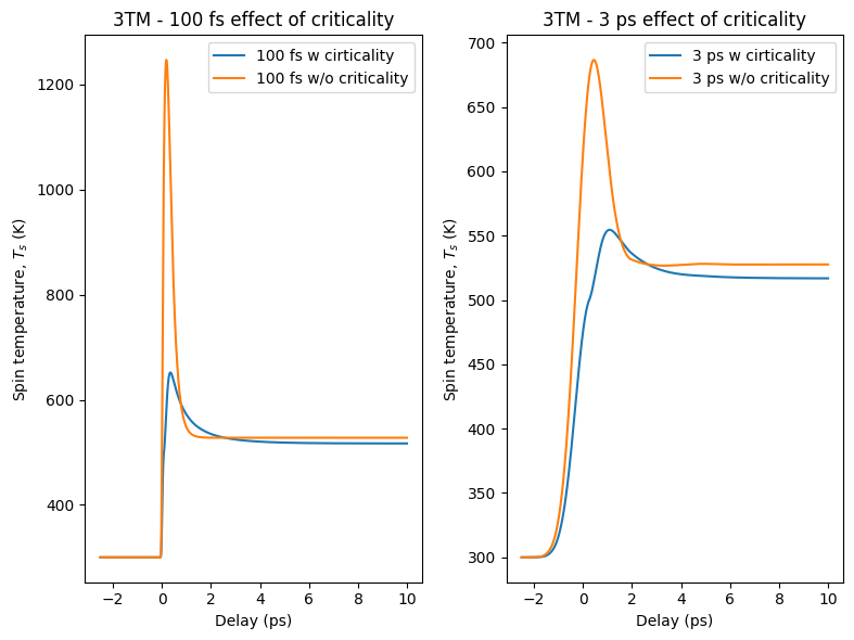
Effect of Criticality#
layer_Co.heat_capacity = [f'{gamma:f}*T',
                          f'(2.98e6 + 1.5e3*(T-300))/{density_effective.magnitude:f}',
                          f'{C_s0:f}'
                          ]

layer_Pt.heat_capacity = [f'{gamma:f}*T',
                          f'(2.98e6 + 1.5e3*(T-300))/{density_effective.magnitude:f}',
                          f'{C_s0:f}'
                          ]
h.excitation = {'fluence': [fluence]*u.mJ/u.cm**2,
                'delay_pump':  [0]*u.ps,
                'pulse_width':  [0.1/2.355]*u.ps,  # from FWHM to sigma
                'multilayer_absorption': True,
                'wavelength': 800*u.nm,
                'theta': 90*u.deg}

temp_map_100fs_wo_crit, delta_temp_100fs_wo_crit = h.get_temp_map(delays, 300)
Surface incidence fluence scaled by factor 1.0000 due to incidence angle theta=90.00 deg
Calculating _heat_diffusion_ for excitation 1:1 ...
Absorption profile is calculated by multilayer formalism with p-polarization.
Total reflectivity of 55.5 % and transmission of 27.9 %.
Elapsed time for _heat_diffusion_ with 1 excitation(s): 29.258881 s
Calculating _heat_diffusion_ without excitation...
Elapsed time for _heat_diffusion_: 24.994643 s
Elapsed time for _temp_map_: 54.358530 s
h.excitation = {'fluence': [fluence]*u.mJ/u.cm**2,
                'delay_pump':  [0]*u.ps,
                'pulse_width':  [3.0/2.355]*u.ps,  # from FWHM to sigma
                'multilayer_absorption': True,
                'wavelength': 800*u.nm,
                'theta': 90*u.deg}

temp_map_3ps_wo_crit, delta_temp_3ps_wo_crit = h.get_temp_map(delays, 300)
Surface incidence fluence scaled by factor 1.0000 due to incidence angle theta=90.00 deg
Calculating _heat_diffusion_ for excitation 1:1 ...
Absorption profile is calculated by multilayer formalism with p-polarization.
Total reflectivity of 55.5 % and transmission of 27.9 %.
Elapsed time for _heat_diffusion_ with 1 excitation(s): 39.144682 s
Calculating _heat_diffusion_ without excitation...
Elapsed time for _heat_diffusion_: 11.097594 s
Elapsed time for _temp_map_: 50.336790 s
Comparison#
plt.figure(figsize=[8, 6])
plt.subplot(1, 2, 1)
plt.plot(delays.to('ps'), np.mean(temp_map_100fs[:, select, 2], 1),
         label='100 fs w cirticality')
plt.plot(delays.to('ps'), np.mean(temp_map_100fs_wo_crit[:, select, 2], 1),
         label='100 fs w/o criticality')
plt.ylabel('Spin temperature, $T_s$ (K)')
plt.xlabel('Delay (ps)')
plt.legend()
plt.title('3TM - 100 fs effect of criticality')

plt.subplot(1, 2, 2)
plt.plot(delays.to('ps'), np.mean(temp_map_3ps[:, select, 2], 1),
         label='3 ps w cirticality')
plt.plot(delays.to('ps'), np.mean(temp_map_3ps_wo_crit[:, select, 2], 1),
         label='3 ps w/o criticality')
plt.ylabel('Spin temperature, $T_s$ (K)')
plt.xlabel('Delay (ps)')
plt.legend()
plt.title('3TM - 3 ps effect of criticality')

plt.tight_layout()
plt.show()